 |
Peano
|
|
Peano
|
Many applications have to touch the solution after each time step: They clip unphysical values such as negative densities, project the solution back onto a constraint manifold, or enforce algebraic constraints of the PDE. ExaGRyPE's CCZ4 formulation of the Einstein equations, for example, requires the conformal metric to have unit determinant and the conformal extrinsic curvature to be trace-free. Such operations are no part of the PDE terms. They are additional steps of the solver, which have to run after each update of the solution.
In this tutorial, we add such a step to the Euler setup of A first advection problem with the Euler equations and Higher-order solvers: Runge Kutta and Finite Differences. We run through the following steps:
We assume that you have completed Higher-order solvers: Runge Kutta and Finite Differences, as we reuse its PDE terms without further explanation.
ExaHyPE does not hard-code what happens within a time step. Instead, the numerical scheme of each solver describes a time step as a task graph (peano4.api.taskgraph.Graph): Each task is one logical step such as "reconstruct the patch with its halo" or "update the cell", and the tasks' dependencies say which step has to finish before another one may start. The ExaHyPE project hands this graph over to a task graph compiler, which maps it onto as few mesh traversals as possible. If you run a script with the logging verbosity TEXT, ExaHyPE prints the task graphs that it hands over to the compiler.
An additional solver step hence is an additional task. It has to be wired into the graph such that it reads the new solution once this solution has been computed, and before anybody else reads it. For the Finite Volumes, this means after the cell update, but before the solution is projected onto the faces, where the neighbours pick it up, and before the CFL condition of the next time step is evaluated.
As in the previous tutorials, we add Peano's Python API to the search path:
The project and the solver are those of Higher-order solvers: Runge Kutta and Finite Differences. The only difference is that the numerical scheme is an instance of a subclass of one of ExaHyPE's schemes, which adds the additional step. We start with the Finite Volumes.
Our additional step is a density floor: Whenever the density in a volume drops below a minimum density, we raise it to this minimum and keep the velocity and the pressure. This is a crude version of the positivity fixes that many codes use to keep densities and pressures positive. To see an effect, we pick an unrealistically high floor of 0.9. Our density wave oscillates between 0.8 and 1.2, i.e. the floor cuts off its troughs.
To insert the step, we have to find the tasks which update the solution. We do not want to know how a particular numerical scheme builds its graph, though. The schemes therefore tag the relevant tasks. Every task (peano4.api.taskgraph.Task) carries a set of tags, i.e. of plain strings, which the task graph compilers ignore. Each numerical scheme adds the tag exahype2.api.Solver.SolutionUpdateTaskTag to every task which writes a new solution. Runge-Kutta schemes add exahype2.api.Solver.IntermediateSolutionUpdateTag to every task which writes the input of a further stage, i.e. an intermediate solution.
Inserting a step then always follows the same pattern:
The place to do this is the numerical scheme: Its routine construct_output() builds the time stepping graph. We subclass the scheme, call the superclass' construct_output() to get the original graph, and then insert our step. The scheme is the right place, as it decides on the data structures: It knows which patch its tagged tasks write and which cells they update. We write the insertion as a plain function, so we can reuse it for further schemes, and let the subclass pass in the patch:
A few details are worth a closer look:
If you want to insert several steps after the same anchor, chain them: Use the task which you have just inserted as the anchor of the next one.
With the class at hand, we create the solver as in the previous tutorials, but use RusanovWithDensityFloor as its numerical scheme:
The remaining steps are the same as in the previous tutorials:
Among the output, you find the time stepping task graph twice: once as the numerical scheme has created it, and once with the density floor. The picture below shows the latter:
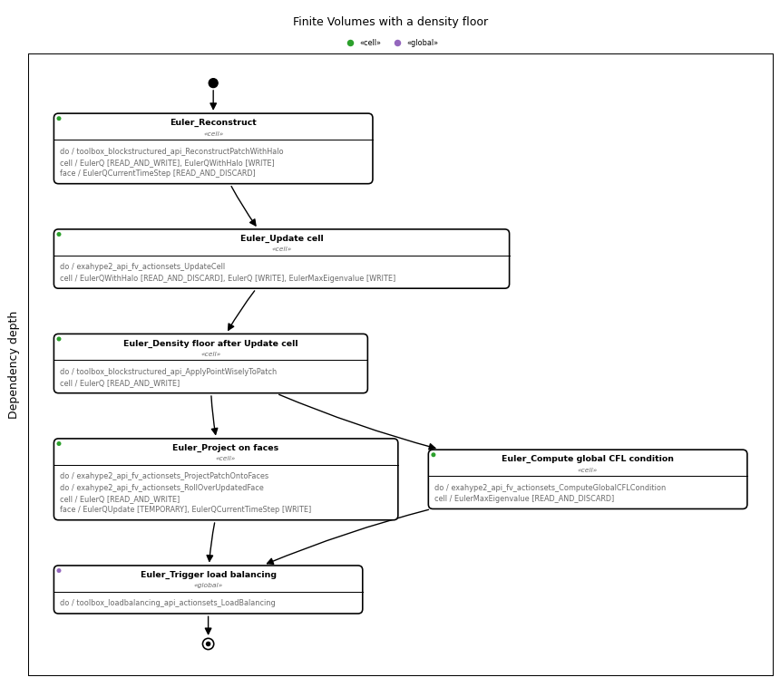
The task "EulerFV_Density floor after Update cell" sits directly behind the cell update. All tasks which used to depend on the cell update, i.e. the projection onto the faces and the evaluation of the CFL condition, now depend on the density floor. Whether the new task costs an additional mesh traversal is up to the task graph compiler. The default compiler maps each task onto a mesh traversal of its own. The new task reads and writes cell data only, though, so a fusing compiler such as peano4.api.taskgraph.compiler.FuseSteps merges it into the mesh traversal of the cell update.
We build and run the code:
After the first time step, the troughs of the wave are flat: The density never drops below 0.9.
A Runge-Kutta scheme does not compute the new solution in one go. It computes a sequence of intermediate solutions, the stages, and evaluates the right-hand side of the PDE for each of them (Higher-order solvers: Runge Kutta and Finite Differences). If we postprocessed the final solution only, the right-hand side would be evaluated for stages which violate our constraints. For a density floor, a stage could even carry a negative density, which the flux cannot handle. The postprocessing therefore has to run after each stage, too.
The Runge-Kutta scheme exahype2.api.rkfd4.CentralDifferencesWithRungeKutta writes the inputs of the further stages into the patch _stage_input and tags these writers with exahype2.api.Solver.IntermediateSolutionUpdateTag. Its subclass hence calls our function twice, once per tag, and passes in the respective patch:
If we switch to the Finite Differences with Runge-Kutta time stepping solver.numerical_scheme = RungeKuttaWithDensityFloor(solver, patch_size=patch_size, rk_order=2) solver.grid_construction = exahype2.api.rkfd4.SetupSimulationOverRegularGrid(solver, volume_size=volume_size) solver.plotter = exahype2.api.rkfd4.PlotAsVTKFile(solver, first_plot_time_stamp=0.0, time_in_between_plots=0.05) the task graph below results. We use a Runge-Kutta scheme of order two to keep the picture small:
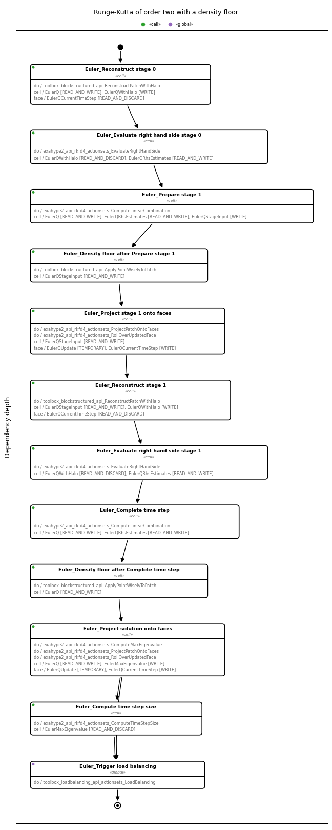
The density floor now runs twice per time step: After "Prepare stage 1", which computes the input of the second stage, and after "Complete time step", which computes the new solution. In both cases, it runs before the outcome is projected onto the faces. The neighbours hence see the postprocessed data only.
The picture below compares the density along \( y=0\) after one period for both schemes, with and without the floor:
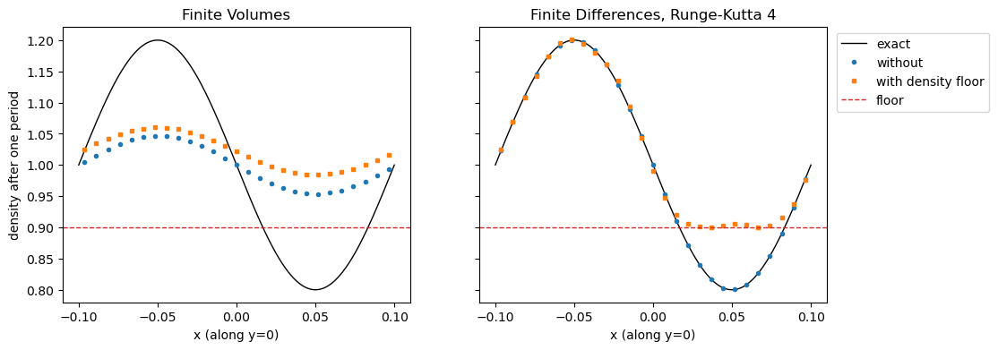
With Runge-Kutta, the floor cuts off the trough of the wave, while the rest of the wave remains on top of the exact solution. After one period, the smallest density is exactly 0.9: The floor holds for every stage, not only for the final solution of each time step.
The floor adds mass whenever it raises the density, i.e. the scheme is no longer conservative. For the Finite Volumes, this is particularly visible: Their numerical diffusion damps the wave such that it stays above the floor after a few time steps. Until then, however, the floor has added mass, and the whole profile ends up above the profile without floor. A density floor hence is a last resort which keeps a code alive, not a physical model. Constraint enforcement is different: It removes errors which the exact solution would not have in the first place.
The tags are a contract between the numerical schemes and any code which inserts steps. The numerical schemes have to tag all tasks which write a new solution or an intermediate solution with the respective tag, and they must not read this solution within the same task. This is why the Runge-Kutta scheme splits the computation of each stage into two tasks, "Prepare stage k" and "Project stage k onto faces": the postprocessing has to fit in between. If a scheme computes the new solution in several tasks, as the optimistic Finite Volumes exahype2.api.fv.RusanovWithOptimisticExplicitEuler do, it tags each of them. Manipulate an existing solver's steps (e.g. inserting additional sweeps) discusses the details.
You can use tags for your own purposes, too: Add any string to a task's set tags and search for it via find_tasks(). Prefix your tags, e.g. with the name of your library, so they cannot clash with the tags of others.
 1.9.8