 |
Peano
|
|
Peano
|
In A first advection problem with the Euler equations, we transported a smooth density wave through a periodic box with Finite Volumes. The error shrank linearly with the mesh width, i.e. the Rusanov scheme with explicit Euler time stepping is a first-order scheme. In this tutorial, we keep the PDE and the setup, but swap the numerical scheme for fourth-order Finite Differences with explicit Runge-Kutta time stepping. ExaHyPE offers this scheme through the package exahype2.api.rkfd4.
We run through the following steps:
We assume that you have completed A first advection problem with the Euler equations, as we reuse its PDE and its setup without further explanation.
Like the Finite Volumes, rkfd4 equips each mesh cell with a patch of \( p \times p\) grid cells and stores the unknowns in the grid cells' centres. Different to the Finite Volumes, there is no Riemann solver. Instead, the scheme reads the PDE \( \partial_t Q + \nabla \cdot F(Q) = 0\) as an ordinary differential equation \( \partial_t Q = R(Q)\) per grid cell, and it evaluates the right-hand side \( R\) through fourth-order central differences of the flux. Along the x-axis, this reads
\begin{eqnarray*} \partial_x F_i \approx \frac{F_{i-2} - 8 F_{i-1} + 8 F_{i+1} - F_{i+2}}{12 h}. \end{eqnarray*}
The stencil reaches into the neighbouring patches. Therefore, ExaHyPE surrounds each patch with a halo of two grid cells, which it fills with data from the neighbours.
The time integration is an explicit Runge-Kutta scheme of order one to four. A Runge-Kutta scheme of order \( s \leq 4\) evaluates \( R\) \( s\) times per time step, each time for a different intermediate solution, the so-called stages. As every stage needs the halo data of the previous stage, ExaHyPE runs through the mesh once per stage: A time step of the fourth-order Runge-Kutta scheme costs roughly four times as much as one explicit Euler step, i.e. a Runge-Kutta step of order one.
Runge Kutta summarises the maths behind Runge-Kutta, and exahype2.api.rkfd4.CentralDifferencesWithRungeKutta documents the realisation within ExaHyPE.
As in the previous tutorials, we add Peano's Python API to the search path:
The project and the solver are the same as in A first advection problem with the Euler equations. We only pick a different directory, namespace and executable name. This time, we do not fill a C++ file with the physics, but hand over the C++ implementation of the flux, the maximum eigenvalue and the initial condition as strings, as discussed at the end of A first advection problem with the Euler equations. The code snippets are the reference implementation of the Euler tutorial.
In A first advection problem with the Euler equations, three lines picked the Finite Volumes: the numerical scheme, the grid construction and the plotter: solver.numerical_scheme = exahype2.api.fv.RusanovWithExplicitEuler(solver, patch_size) solver.grid_construction = exahype2.api.fv.SetupSimulationOverRegularGrid(solver, volume_size=volume_size) solver.plotter = exahype2.api.fv.PlotAsVTKFile(solver, first_plot_time_stamp=0.0, time_in_between_plots=0.005) To switch to the fourth-order Finite Differences, we take these three classes from the package exahype2.api.rkfd4 instead of exahype2.api.fv, and replace the Rusanov scheme with CentralDifferencesWithRungeKutta. Nothing else changes: the PDE terms, the global simulation parameters and the build remain exactly the same.
A few remarks on the arguments:
The grid construction is the same as for the Finite Volumes: volume_size is the maximum size of a grid cell. With 0.0075 and \( 9 \times 9\) grid cells per patch, ExaHyPE ends up with \( 3 \times 3\) patches, i.e. \( 27 \times 27\) grid cells. This is three times coarser than the mesh of A first advection problem with the Euler equations.
These steps are the same as in A first advection problem with the Euler equations. We simulate one period of the wave, i.e. until \( t=0.2\) . If you look at the task graphs that ExaHyPE prints, you see that a time step now consists of one mesh traversal per Runge-Kutta stage.
The code runs a bit more than 250 time steps and writes its snapshots into 12_higher-order-solvers/solution-EulerFD4.peano-patch-file. The viewer of A first advection problem with the Euler equations works for the Finite Differences, too:
Different to the Finite Volumes, you will not spot any loss of amplitude, even though our mesh is three times coarser than the one of A first advection problem with the Euler equations.
We know the exact solution, so we can measure the error directly. The function below reads the last snapshot, compares the density in each grid cell centre with the exact density and returns the maximum difference.
There is one technical detail: The patch files hold the patches' offsets with seven significant digits only, as they are meant for visualisation. Errors below roughly \( 10^{-7}\) would therefore be dominated by the imprecise grid cell positions. As we know that the mesh is regular, we snap the offsets onto the mesh.
After one period, the maximum error on \( 27 \times 27\) grid cells is around \( 1.2 \cdot 10^{-4}\) . The Finite Volumes of A first advection problem with the Euler equations end up with an error around \( 0.15\) on the same mesh. The picture below compares the two schemes along the line \( y=0\) :
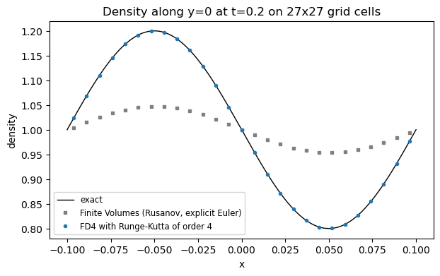
The Finite Volumes lose a big part of the wave's amplitude due to their numerical diffusion, while the Finite Differences remain on top of the exact solution.
To determine the order of a scheme, we run it on a sequence of meshes and see how fast the error shrinks. We use the volume sizes 0.0075, 0.0025 and 0.00083, i.e. \( 27 \times 27\) , \( 81 \times 81\) and \( 243 \times 243\) grid cells. Each mesh is three times finer than its predecessor, so a scheme of order \( k\) should reduce the error by a factor of \( 3^k\) from one mesh to the next. To keep the runs short, we stop at \( t=0.05\) . The table lists the maximum error of the density:
| Scheme | \( 27 \times 27\) | \( 81 \times 81\) | \( 243 \times 243\) | Observed order |
|---|---|---|---|---|
| Finite Volumes (Rusanov, explicit Euler) | \( 6.2 \cdot 10^{-2}\) | \( 2.4 \cdot 10^{-2}\) | \( 8.4 \cdot 10^{-3}\) | 0.87, 0.95 |
| FD4 with Runge-Kutta of order 1 | \( 4.0 \cdot 10^{-3}\) | \( 1.3 \cdot 10^{-3}\) | \( 1.2 \cdot 10^{-3}\) | 1.00, 0.08 |
| FD4 with Runge-Kutta of order 2 | \( 2.2 \cdot 10^{-6}\) | \( 3.3 \cdot 10^{-6}\) | \( 4.0 \cdot 10^{-7}\) | -0.35, 1.91 |
| FD4 with Runge-Kutta of order 3 | \( 3.0 \cdot 10^{-5}\) | \( 3.8 \cdot 10^{-7}\) | \( 4.7 \cdot 10^{-9}\) | 3.99, 4.00 |
| FD4 with Runge-Kutta of order 4 | \( 3.0 \cdot 10^{-5}\) | \( 3.8 \cdot 10^{-7}\) | \( 4.7 \cdot 10^{-9}\) | 3.99, 4.00 |
The picture shows the same data. The dotted grey lines are reference slopes of order one, two and four:
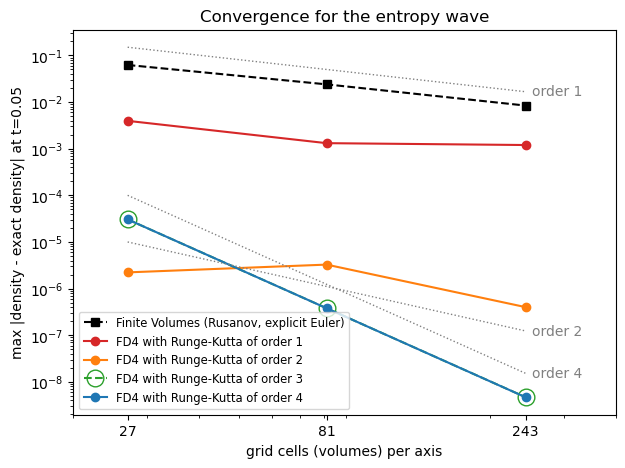
The Finite Volumes converge with order one: Every refinement reduces the error by a factor of roughly three. The Finite Differences with the fourth-order Runge-Kutta scheme converge with order four, i.e. each refinement reduces the error by a factor of \( 3^4 = 81\) . On the coarsest mesh, they are already more accurate than the Finite Volumes on the finest mesh, although the latter has 81 times more grid cells and needs almost five times more time steps.
The Finite Differences are of fourth order in space. The time step size is proportional to the mesh width \( h\) due to the CFL condition. A Runge-Kutta scheme of order \( s\) hence contributes an error of \( \mathcal{O}(\Delta t^s) = \mathcal{O}(h^s)\) , and we expect the overall error to behave like
\begin{eqnarray*} e \approx C_x h^4 + C_t h^s. \end{eqnarray*}
Asymptotically, i.e. for very fine meshes, the smaller of the two orders wins. For the meshes that we can afford, the constants \( C_x\) and \( C_t\) matter, too. The table and the picture above show what this means in practice:
So the Runge-Kutta scheme makes a limited difference as long as it is accurate enough: Its order has to be high enough that the time stepping error does not dominate the error of the spatial discretisation. Beyond that point, a higher order only increases the cost.
On the finest mesh, explicit Euler yields an error convergence order well below one. The picture below shows what is going on. It runs the scheme with explicit Euler, Runge-Kutta of order two and of order four on \( 81 \times 81\) grid cells for a whole period. The left plot shows the maximum error over time, the right plot shows the error along \( y=0\) at the end of the simulation with explicit Euler:
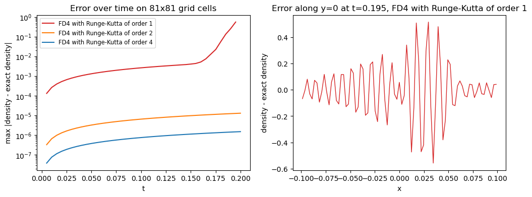
For most of the simulation, the error of explicit Euler grows linearly, as we would expect from a first-order time integrator. Towards the end, it explodes. The right plot shows why: The solution is polluted by an oscillation on the scale of the grid cells, i.e. by the highest frequencies that the mesh can represent.
Central differences do not add any numerical diffusion. For a linear advection \( \partial_t Q + a \partial_x Q = 0\) , the right-hand side of each Fourier mode \( \hat Q e^{i k x}\) is purely imaginary, \( R = i \omega \hat Q\) , where the frequency \( \omega\) is proportional to \( a/h\) for the highest frequencies. One explicit Euler step multiplies such a mode by
\begin{eqnarray*} |1 + i \omega \Delta t| = \sqrt{1 + (\omega \Delta t)^2} > 1, \end{eqnarray*}
i.e. every mode grows, no matter how small we choose the time step size. The highest frequencies grow fastest. They start from round-off errors around \( 10^{-15}\) , so they need several hundred time steps of growth by a few percent to become visible. On \( 81 \times 81\) grid cells, one period takes around 760 time steps, so the instability kicks in before the end of the simulation. On \( 27 \times 27\) grid cells, one period needs only about 250 time steps, and the instability remains invisible, although it is there. The finer the mesh, the more time steps we need, and the earlier the simulation breaks down.
Runge-Kutta of order two is not stable for purely imaginary eigenvalues either, but its growth factor per step, \( \sqrt{1 + (\omega \Delta t)^4/4}\) , is so close to one that we do not see the instability within one period. The schemes of order three and four are stable as long as \( \omega \Delta t\) is not too big, which the CFL condition ensures.
The Finite Volumes of A first advection problem with the Euler equations do not suffer from this problem, although they use explicit Euler, too: The Rusanov flux adds numerical diffusion, which damps the highest frequencies. This is exactly the numerical diffusion that smears out the wave. Use the Finite Differences with Runge-Kutta of order three or four.
The pictures of this tutorial are created by the script tutorials/exahype2/illustrations/12_higher-order-solvers.py, which runs all the experiments above. The fourth-order convergence benchmark uses the same setup with Dirichlet boundary conditions and in two or three dimensions.
 1.9.8