 |
Peano
|
|
Peano
|
This is the first tutorial on how to model a PDE with ExaHyPE 2. We solve the compressible Euler equations for a very simple scenario: a smooth density wave which is transported through a periodic box. As we know the exact solution, we can always check if what ExaHyPE computes is correct. The setup is the same as in the smooth convergence test benchmark, i.e. once you have completed this tutorial, you should be able to read and modify the benchmark's script.
We run through the following steps:
The compressible Euler equations describe the conservation of the density \( \rho\) , the momentum \( \rho u\) and the total energy \( E\) of an ideal gas. In two dimensions, they read
\begin{eqnarray*} \frac{\partial}{\partial t} \begin{pmatrix} \rho \\ \rho u_1 \\ \rho u_2 \\ E \end{pmatrix} + \nabla \cdot \begin{pmatrix} \rho u_1 & \rho u_2 \\ \rho u_1^2 + p & \rho u_1 u_2 \\ \rho u_2 u_1 & \rho u_2^2 + p \\ (E + p)u_1 & (E + p)u_2 \end{pmatrix} = \vec{0}. \end{eqnarray*}
The pressure follows from the equation of state of an ideal gas
\begin{eqnarray*} p = (\gamma - 1)\left(E - \frac{1}{2}\rho(u_1^2 + u_2^2)\right) \end{eqnarray*}
with \( \gamma = 1.4\) (dry air). The speed of sound is \( c = \sqrt{\gamma p / \rho}\) , and the eigenvalues of the flux in direction \( n\) are \( u_n - c\) , \( u_n\) and \( u_n + c\) . ExaHyPE needs the largest of them in absolute value, as it determines both the numerical flux and the admissible time step size.
There is one pitfall: ExaHyPE stores the conserved quantities \( Q = (\rho, \rho u_1, \rho u_2, E)\) , i.e. density, the two momenta and the energy, but not the velocities. Whenever a formula uses \( u_n\) , we have to divide the momentum by \( \rho\) .
We pick initial conditions where the velocity and the pressure are constant, while the density varies:
\begin{eqnarray*} \rho(x,y,0) = 1 + 0.2 \sin\left( 2\pi \frac{x+0.1}{0.2} \right), \qquad u_1 = 1, \qquad u_2 = 0, \qquad p = 1. \end{eqnarray*}
The domain is the square \( [-0.1,0.1]^2\) with periodic boundary conditions. If you insert this setup into the Euler equations, you find out that pressure and velocity remain constant, and the density is simply transported (advected) with speed \( u_1 = 1\) to the right. Physicists call this an entropy wave. The exact solution is
\begin{eqnarray*} \rho(x,y,t) = 1 + 0.2 \sin\left( 2\pi \frac{x - t + 0.1}{0.2} \right). \end{eqnarray*}
After \( t=0.2\) , the wave has crossed the domain once and is back at its initial position. At the origin, the density is \( \rho(0,0,t) = 1 + 0.2 \sin( 10 \pi t )\) , i.e. an observer sitting at the origin sees a sine over time. We will use this fact at the end of the tutorial.
Even though the Euler equations are non-linear, this solution is smooth. Smooth solutions are exactly what we need to assess how accurate a numerical scheme is. Shocks would hide the scheme's order behind the discontinuity.
The Python API of Peano and ExaHyPE resides within the src directory of your Peano installation. Unless you have installed it via pip install -e ., we add it to the search path manually:
The interactive visualisation at the end of this tutorial needs ipywidgets and matplotlib. If they are not available yet, install them through your preferred package manager or directly from within the notebook:
Every ExaHyPE 2 code starts with a project. The project describes the C++ namespace of the generated code, the name of the executable, and the directory into which all of the generated code goes. We use a subdirectory 10_euler, as the generator produces quite a lot of files and directories.
Next, we create a solver. A solver has a name, which also determines the name of the generated C++ classes and the output files, a number of unknowns, and a number of auxiliary variables. The Euler equations in 2d have four unknowns: \( (\rho, \rho u_1, \rho u_2, E)\) .
The distinction between unknowns and auxiliary variables is important: Only unknowns evolve according to the PDE. Auxiliary variables are not subject to flux, non-conservative product, sources, and so forth. They can hold constants such as material parameters, or helper variables that you update with some other logic. We do not need any of them.
So far, ExaHyPE does not know anything about our PDE. We tell it which terms our PDE consists of. The Euler equations need a flux and the maximum eigenvalue of the flux. Furthermore, we want to set the initial condition point-wisely: ExaHyPE hands us a point \( x\) and we return the solution \( Q(x)\) at \( t=0\) .
We have not given any implementation of these terms. ExaHyPE will therefore generate a C++ class with empty functions for flux, max eigenvalue and initial condition, which we fill later on.
The flag stateless is a performance optimisation: A stateless term does not access any attributes of the solver object. ExaHyPE can then make the C++ function static and offload it to GPUs, e.g. We do not care about performance here, so we keep the default.
We discretise the PDE with Finite Volumes. ExaHyPE groups the finite volumes into patches: Each cell of the Peano mesh carries a patch of \( 9 \times 9\) volumes. The numerical scheme uses a Rusanov flux between neighbouring volumes and explicit Euler in time. It picks the time step size according to the CFL condition
\begin{eqnarray*} \Delta t = 0.9 \cdot \frac{h}{d \cdot \lambda_{max}}, \end{eqnarray*}
where \( h\) is the volume size, \( d\) the dimension, and \( \lambda_{max}\) the largest eigenvalue in the domain.
For the mesh, we use a regular grid. We specify the maximum volume size we accept, and ExaHyPE picks the coarsest regular Peano mesh which delivers volumes that are at most this size. As Peano splits each cell into \( 3 \times 3\) cells whenever it refines, the domain is split into \( 3^k \times 3^k\) patches.
With a volume size of 0.005, ExaHyPE ends up with \( 9 \times 9\) patches, i.e. with \( 81 \times 81\) volumes in total. Each one has a size of \( 0.2/81 \approx 0.0025\) . The picture below shows the initial density on this mesh. The white lines are the patch boundaries, the red box shows the volumes of one patch.
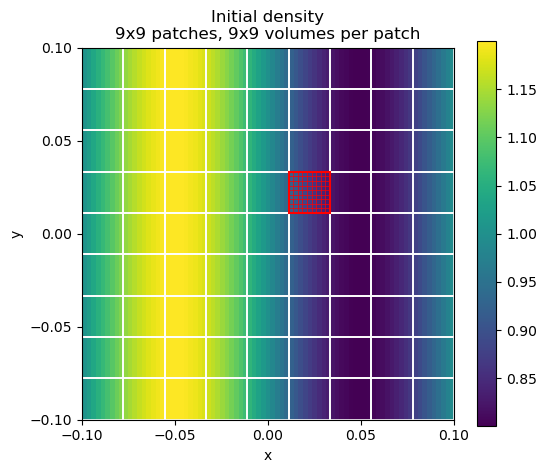
The benchmark uses a volume size of 0.001, which yields \( 27 \times 27\) patches. We stick to the coarser mesh for the time being, as it runs within seconds.
Finally, the solver needs a plotter. The plotter writes the solution in Peano's patch file format: one meta file plus one file per snapshot. We plot every 0.005 time units.
We add the solver to the project and specify the domain, the time span we simulate, and the boundary conditions. We simulate exactly one period of the wave, i.e. until \( t=0.2\) .
Now we lower the ExaHyPE project into a Peano project, and the Peano project into C++ code plus a Makefile. ExaHyPE has to know where Peano is installed, as the Makefile links against Peano's libraries. We pass an absolute path, as the generated Makefile resides in the subdirectory 10_euler. We also pick the release mode. The benchmark uses debug mode, which is way slower but checks many assertions.
If you set the verbosity to TEXT, ExaHyPE prints the task graphs it derives from your solver: one to set up the simulation (construct the mesh, set the initial condition), one per time step, and one to plot.
Let's see what we got:
ExaHyPE and Peano have given us a couple of files and directories:
Let's have a look into the solver class:
There are three functions to fill: flux, maxEigenvalue and initPointWisely. We do not need any boundary conditions, as the domain is periodic.
Open 10_euler/EulerFV.cpp and implement the three functions:
If you want to skip the exercise, run the cell below. It overwrites the file with our reference implementation, which is the same as in the benchmark.
Peano and ExaHyPE can be very chatty. On startup, the executable reads a log filter file which white- or black-lists log messages per level and namespace. If the file is missing, you get a warning and everything is switched on. Debug and trace messages only exist in debug builds anyway, but we want to be explicit:
Peano gives us a good old Makefile, so we compile with make and then run the executable. The first build takes around half a minute.
The code runs a little bit more than 400 time steps and writes 41 snapshots into 10_euler/solution-EulerFV.peano-patch-file plus the files it includes.
The plotter dumps Peano patch files. Peano's plotter package offers a small viewer for Jupyter notebooks. It reads the patch files directly and gives you a time slider, a play button, and a selector for the unknown. The colour range is fixed by the first snapshot, so you can see the wave travelling to the right and losing amplitude.
If you prefer ParaView, convert the patch files into VTU files with Peano's render script. It relies on the ParaView/VTK Python libraries: cd 10_euler python3 ../../../src/tarch/plotter/api/render.py solution-EulerFV.peano-patch-file
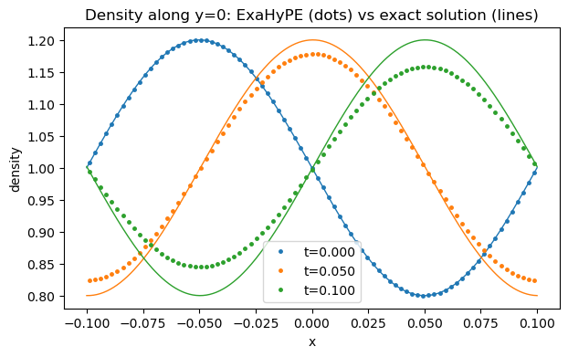
The plot below shows the density along the line \( y=0\) for three time stamps. The lines are the exact solution, the dots are the volume averages computed by ExaHyPE. At \( t=0\) , both match perfectly. Over time, the numerical solution moves at the right speed, but it loses amplitude: the peaks are smeared out. This is numerical diffusion. The Rusanov flux adds artificial viscosity to keep the scheme stable, and the coarser the mesh, the stronger this effect.
Often, we are not interested in the whole solution but in what happens at one particular point over time, e.g. where a sensor sits. Peano's probe script reads the patch files and writes the values at one point over all snapshots into a csv file. There is no interpolation: it takes the value of the finest volume containing the point. We probe the origin and process the snapshots in parallel:
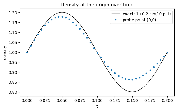
The csv file holds one row per snapshot: the time stamp followed by the four unknowns. We compare the density with the exact solution \( 1 + 0.2 \sin(10 \pi t)\) :
You should get the following picture: The observer at the origin indeed sees a sine. The numerical solution follows it, but with a smaller amplitude, as we have seen before.
The benchmark is called a convergence test, as it is used to check that the numerical error shrinks as expected when we refine the mesh. The Rusanov scheme with explicit Euler is a first-order scheme: If we make the volumes \( k\) times smaller, the error should go down by a factor of \( k\) .
The picture below compares the error at the probe point for our volume size of 0.005 (81 volumes per direction) with the benchmark's volume size of 0.001 (243 volumes per direction). The volumes are three times smaller. The maximum error shrinks from 0.063 to 0.024, i.e. by a factor of 2.6. This is close to the factor of 3 that we expect from a first-order scheme.
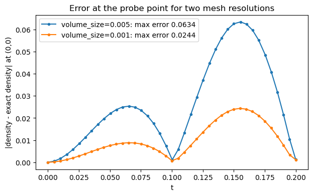
Exercise:** Reproduce this picture. Change the volume size to 0.001, rerun the notebook from the cell where we set up the mesh, and compare the two csv files. Your C++ implementation in EulerFV.cpp is not overwritten when you regenerate the code.
The pictures of this tutorial are created by the script tutorials/exahype2/illustrations/10_euler.py, which runs exactly this experiment for both volume sizes.
Instead of editing EulerFV.cpp, you can hand the C++ implementation of a PDE term over as a string. ExaHyPE then writes it into the generated code directly, and you do not have to touch any C++ file. The benchmark's script smooth-convergence-test-with-injected-functions.py follows this route: solver.add_pde_term( exahype2.api.Flux( implementation = ''' const double irho = 1.0 / Q[0]; ... ''', stateless = False, ) ) This is convenient for small terms or if you generate the C++ code with SymPy, e.g. For larger projects, a proper C++ file is usually easier to maintain and debug.
 1.9.8