While most users might be fine with the time stepping schemes offered by ExaHyPE and the idea that they only attach a numerical scheme to a physical model, developers of numerical schemes as well as some advanced PDEs might have to manipulate the solver's task graph. Examples are the enforcement of the CCZ4 constraints or a density floor for the Euler equations, i.e. particular PDEs subject to constraints. The tutorial Additional solver steps: postprocessing the solution after each update runs through such a hands-on example. This page discusses the underlying mechanics.

From a solver to task graphs

Every exahype2.api.Solver contributes to three task graphs (peano4.api.taskgraph.Graph), one per algorithmic phase: the setup of the simulation, the time stepping, and the plotting. When the project generates the code, it calls each solver's generate_solver_realisation(), which proceeds in three steps:

The grid construction (exahype2.api.Solver.GridConstruction) adds its tasks to the setup graph.
The numerical scheme (exahype2.api.Solver.NumericalScheme) adds its tasks to the time stepping graph.
The plotter (exahype2.api.Solver.Plotter), if any, adds its tasks to the plot graph.

Each of the three does so in its routine construct_output(), which receives the respective graph. Only afterwards, the project hands the graphs over to the task graph compiler. The graphs are shared by all solvers of a project, i.e. the time stepping graph also holds the tasks of the solvers which have been processed before.

There is no solver-wide hook which receives the complete graphs. You might want to modify a solver's task graph agnostic of its numerical scheme, but this is rarely possible:

It will not always be possible (and desirable) to modify a task graph in a numerical scheme agnostic way. Therefore, you do not plug into a solver's task graph construction, but into the numerical scheme's task graph construction (generator) itself. This is also, in many cases, the better way to go, as the numerical scheme decides on the data structures used.

So we summarise: The way to get your own postprocessing into a solver's time stepping is to subclass the numerical scheme and extend its construct_output() routine: Call the superclass' construct_output() to get the original task graph, and then add your own tasks to it. At this point, all tasks of the scheme are known, but none of them has been translated into a grid traversal yet. If you want to alter the setup or the plot graph, subclass the grid construction or the plotter, respectively, in the same way.

Tags

Tags are a mechanism to, well, tag particular tasks. They carry no semantics in themselves (at least none imposed by Peano) but allow people to find particular tasks within a task graph. This is convenient for ExaHyPE, as we want, in an ideal world, to modify a task graph while at the same time not interfering with the actual task graph construction itself.

Different numerical schemes will define different tags, and you have to look up which tags, i.e. particular plug-in points a scheme introduces, but there are a few standard tags which all schemes should support:

The solution update tags

exahype2.api.Solver defines two tags, i.e. two string constants:

exahype2.api.Solver.SolutionUpdateTaskTag: Each numerical scheme of ExaHyPE adds this tag to each task of its time stepping graph which writes a new solution.
exahype2.api.Solver.IntermediateSolutionUpdateTag: Runge-Kutta schemes compute intermediate solutions, i.e. the inputs of further stages, before they compute the new solution. They add this tag to each task which writes such an intermediate solution.

No task carries both tags. For an explicit single-step scheme such as exahype2.api.fv.RusanovWithExplicitEuler, the task which writes the new solution carries exahype2.api.Solver.SolutionUpdateTaskTag only, and no task carries exahype2.api.Solver.IntermediateSolutionUpdateTag. For multi-stage schemes such as Runge-Kutta, several tasks will hold exahype2.api.Solver.IntermediateSolutionUpdateTag, but only one, the task after the last stage, will carry exahype2.api.Solver.SolutionUpdateTaskTag. As the tags are disjoint, each of them also identifies the data which the tagged tasks write: For exahype2.api.rkfd4.CentralDifferencesWithRungeKutta, the tasks with SolutionUpdateTaskTag write the solution solver._patch, the tasks with IntermediateSolutionUpdateTag write the stage input solver._stage_input.

The distinction allows you to pick: A step which should act on the solution only, e.g. some statistics, searches for SolutionUpdateTaskTag. A step which should act on every intermediate solution, too, e.g. the enforcement of constraints or a density floor, searches for both tags.

Inserting steps

Inserting a step always follows the same pattern: Call find_tasks(), and, for each task returned, create a new task and add it to the graph via insert_after(). The sketch below adds a density floor after each update of a Runge-Kutta scheme:

class MySolversRungeKuttaScheme(exahype2.api.rkfd4.CentralDifferencesWithRungeKutta):
  def construct_output(self, exahype2_project, peano_project, time_step):
    ## Adds the scheme's tasks to time_step
    super().construct_output(exahype2_project, peano_project, time_step)
    solver = self._solver
    for tag, patch in [
      (exahype2.api.Solver.SolutionUpdateTaskTag,         solver._patch),
      (exahype2.api.Solver.IntermediateSolutionUpdateTag, solver._stage_input),
    ]:
      for anchor in time_step.find_tasks(tag):
        ## The graph holds the tasks of all solvers
        if not anchor.name.startswith(solver.name + "_"):
          continue
        new_intermediate_task = peano4.api.taskgraph.Task(
          name   = f"{solver.name}_Density floor after {anchor.name[len(solver.name) + 1:]}",
          entity = peano4.api.taskgraph.Task.GridEntity.CELL,
        )
        new_intermediate_task.use_cell(patch, peano4.api.taskgraph.Task.DataAccess.READ_AND_WRITE)
        new_intermediate_task.add_action_set(
          toolbox.blockstructured.api.ApplyPointWiselyToPatch(
            patch               = patch,
            implementation      = "Q[0] = std::max(Q[0], 0.9);",
            guard               = solver.grid_selector.createCellGuard(),
            additional_includes = solver._get_default_includes() + solver.user_solver_includes,
          )
        )
        ## Adds the task to the graph, i.e. this routine is
        ## responsible that new_intermediate_task has an in-dependency
        ## on anchor, and all of anchor's outgoing dependencies are
        ## rewired into new_intermediate_task.
        time_step.insert_after(anchor, new_intermediate_task)

You then use the subclass instead of the original scheme:

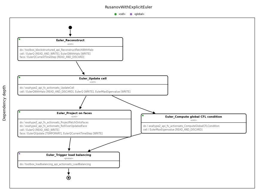
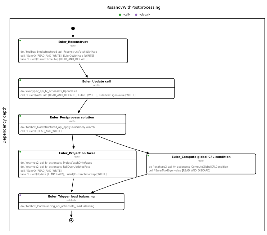
solver.numerical_scheme = MySolversRungeKuttaScheme(solver, patch_size=9, rk_order=2)

What happens: the Rusanov solver

The pictures below show the effect of such a subclass for the Finite Volumes exahype2.api.fv.RusanovWithExplicitEuler. Here, only the task "Update cell" carries a tag, i.e. exahype2.api.Solver.SolutionUpdateTaskTag, and it writes the solution solver._patch. The subclass therefore searches for this one tag:

class RusanovWithPostprocessing(exahype2.api.fv.RusanovWithExplicitEuler):
  def construct_output(self, exahype2_project, peano_project, time_step):
    super().construct_output(exahype2_project, peano_project, time_step)
    solver = self._solver
    for anchor in time_step.find_tasks(exahype2.api.Solver.SolutionUpdateTaskTag):
      if not anchor.name.startswith(solver.name + "_"):
        continue
      task = peano4.api.taskgraph.Task(
        name   = f"{solver.name}_Postprocess solution",
        entity = peano4.api.taskgraph.Task.GridEntity.CELL,
      )
      task.use_cell(solver._patch, peano4.api.taskgraph.Task.DataAccess.READ_AND_WRITE)
      task.add_action_set(
        toolbox.blockstructured.api.ApplyPointWiselyToPatch(
          patch               = solver._patch,
          implementation      = "Q[0] = std::max(Q[0], 0.9);",
          guard               = solver.grid_selector.createCellGuard(),
          additional_includes = solver._get_default_includes() + solver.user_solver_includes,
        )
      )
      time_step.insert_after(anchor, task)

The original time stepping graph of the scheme on the left, and the graph of the subclass on the right:

In the original graph, two tasks depend on "Update cell": the projection onto the faces, which hands the new solution over to the neighbours, and the evaluation of the CFL condition, which reduces the maximum eigenvalues into the next time step size. insert_after() makes the new task depend on "Update cell" and rewires both successors to the new task. Consequently, the neighbours see the postprocessed solution only. Whether the new task costs an additional mesh traversal is up to the task graph compiler. The default compiler of exahype2.api.Project, peano4.api.taskgraph.compiler.Sequential, maps each task onto a traversal of its own, i.e. the time step grows from five to six traversals. The new task reads and writes cell data only, so a fusing compiler such as peano4.api.taskgraph.compiler.FuseSteps merges it into the traversal of the cell update: It needs two traversals per time step with and without the new task.

Note that the CFL condition does not read the solution: "Update cell" writes the maximum eigenvalue alongside the solution, and it computes it from the Riemann problems of the update, i.e. from the old solution. The new task hence does not alter the next time step size. The pictures are created by documentation/exahype2/programmers-guide/manipulate-solver-steps-illustrations.py.

Comments on this particular example

toolbox.blockstructured.api.ApplyPointWiselyToPatch runs a C++ snippet for each volume, or grid point, of a patch. The snippet may read and write Q, i.e. all unknowns and auxiliary variables of one volume, and read the volume's position x. Your step can use any other action set as well, e.g. one which needs a halo or works on faces or vertices.

Declare the patch with READ_AND_WRITE even if your step only reads it: the access mode keeps the data alive for the tasks which follow. Drop the IntermediateSolutionUpdateTag entry from the loop if your step should run once per time step only, i.e. not after each Runge-Kutta stage.

Some schemes write the new solution in several tasks, of which each cell runs exactly one. The optimistic Finite Volumes exahype2.api.fv.RusanovWithOptimisticExplicitEuler, for example, tag both "Update cell" and "Insert patch interior" with SolutionUpdateTaskTag, i.e. the two tasks which complete a time step, but not the partial updates of the patch shell or interior. Inserting one step after each of them with the plain cell guard would run the step twice for the cells of the optimistic branch. Pass all tagged tasks of your solver to insert_after() instead: insert_after([update_cell, insert_patch_interior], task) makes task depend on both and rewires the successors of both to task. task then runs once per cell, after whichever of the two has completed the time step of this cell. exagrype.api.CCZ4Solver inserts its constraint enforcement this way.

The numerical scheme's construct_output() receives the time stepping graph only. The tags are only used within this graph, too. If you want to alter the setup or the plot graph, subclass the grid construction or the plotter, identify the tasks of interest yourself, e.g. via their names, or add tasks which do not depend on any existing task.