 |
Peano
|
|
Peano
|
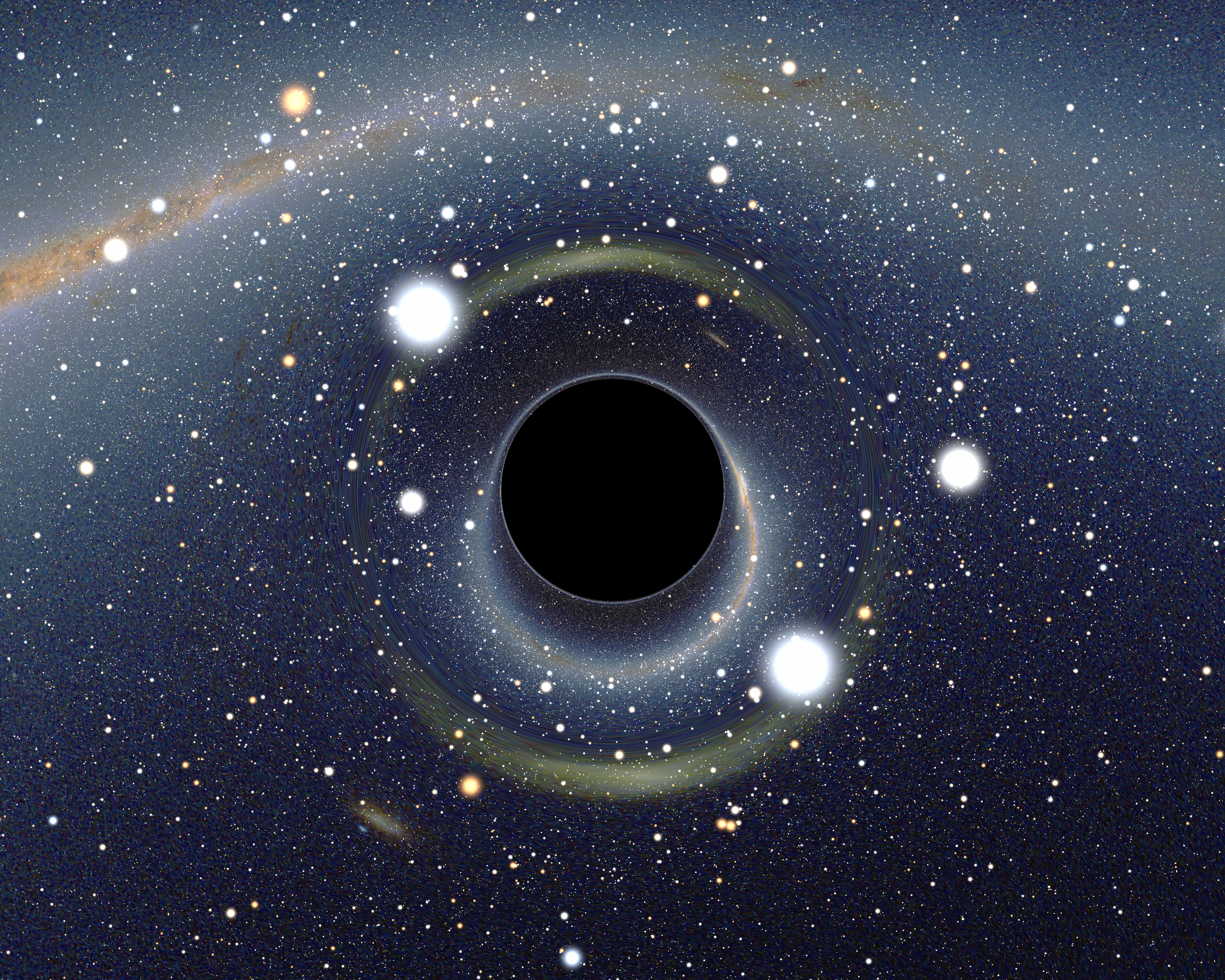
This tutorial simulates a single, non-spinning black hole with ExaGRyPE. It is the second step after The gauge wave: A first numerical relativity experiment with ExaGRyPE. The gauge wave is flat spacetime in disguise, while we now evolve a spacetime with a genuine singularity. At the same time, the tutorial documents how we built the first version of the benchmark Single Schwarzschild black hole with the new Python API exagrype.api.
We run through the following steps:
Before you start, configure and build Peano as described in Configure ExaGRyPE. Different to the gauge wave, you need the GNU Scientific Library (GSL), i.e. you have to configure with --with-gsl on top of --enable-exagrype. TwoPunctures, which computes our initial data, relies on it.
We simulate the Schwarzschild solution, i.e. a black hole of mass \( M\) which neither moves nor spins. In isotropic coordinates, its spatial metric is conformally flat:
\begin{eqnarray*} \gamma_{ij} = \psi^4 \delta_{ij}, \qquad \psi(r) = 1 + \frac{M}{2r}. \end{eqnarray*}
The conformal factor \( \psi\) diverges at \( r=0\) . This point is called the puncture. ExaGRyPE uses the puncture method: Rather than cutting the black hole out of the domain (excision), it evolves the singular data and relies on the gauge, i.e. on lapse and shift, to keep the numerical solution under control around the puncture. Inside the black hole, the details of the solution do not matter, as no information escapes through the horizon at \( r = M/2\) . The price to pay is a high resolution requirement around the puncture.
We place the black hole with \( M=1\) at the origin of the domain \( [-9,9]^3\) . The data is not exactly what an analytical formula gives us: Black hole simulations typically obtain their initial data from TwoPunctures, a solver for binary black hole initial data from the Einstein Toolkit. For a single black hole, we set the mass of the second black hole to zero. We will check below that TwoPunctures then indeed reproduces the formula above.
What do we expect? The black hole is stationary, but our coordinates are not adapted to it: The lapse and the shift evolve until they settle into a stationary gauge. The system should hence become (quasi-)static after some time, with the black hole staying at the origin. A real production run therefore runs for a long time and checks that the black hole stays where it is and that the solution settles down.
As in the gauge wave tutorial, we add the Python API to the search path and memorise the Peano root directory.
The initial condition of an exahype2.api.Solver is an exahype2.api.InitPointWisely term: a C++ snippet which receives the position x of one degree of freedom and writes the initial values of all unknowns into Q. For the gauge wave, this snippet calls an analytical formula from the ExaGRyPE library. TwoPunctures is different, as it is a solver of its own: It first has to solve an elliptic equation on a spectral grid. Afterwards, we can interpolate its solution at any point x.
Rather than generating the setup of TwoPunctures from Python, we moved all of this logic into the ExaGRyPE library itself: exagrype::initialvalues::singleBlackHole() (in src/exagrype/initialvalues/ApplyTwoPunctures.h). The routine
The Python counterpart exagrype.api.initialvalues.single_black_hole() then is a one-liner: It returns an InitPointWisely term which calls the C++ routine. Let's look at the C++ snippet it produces:
TwoPunctures only becomes part of the ExaGRyPE library if Peano is configured with GSL. Otherwise, the snippet stops the compilation with a meaningful error message rather than an obscure linker error.
This is a pattern which we will see over and over again: Whenever the generated code would contain more than a call or two, we write the logic as a plain C++ function in the library, and the Python API only generates the call. The C++ code then can be read, debugged and unit tested like any other C++ code.
We create the CCZ4 solver as for the gauge wave, but hand in the black hole initial condition. We also change two parameters: We switch on the evolution of the shift (CCZ4sk), i.e. the Gamma driver, and the advection terms within this driver (CCZ4bs). The gauge wave keeps the shift at zero and hence does not need either of them. All other parameters keep their defaults. In particular, CCZ4LapseType=0 selects harmonic slicing.
The gauge wave lives on a periodic domain. The black hole does not: Our domain \( [-9,9]^3\) cuts out a finite piece of an infinite spacetime, and we have to tell the code what happens at its boundary. As soon as at least one axis is not periodic, exahype2.api expects the solver to have exactly one boundary condition term: either an exahype2.api.DirichletBoundaryConditions or an exahype2.api.SommerfeldBoundaryConditions term. The Dirichlet term receives the position x of a ghost volume outside of the domain and a time stamp t, and it has to write the solution there into Q.
Black hole codes typically use Sommerfeld conditions, which we discuss at the end of this tutorial. They assume that all fields approach their values at infinity like outgoing waves, i.e. they let waves leave the domain with little reflection. Sommerfeld conditions need the solution inside the domain and the normal of the boundary face. The Dirichlet term of the new API receives neither of them. For a first version, we hence take the simplest option that is consistent with our setup: We hold the boundary at the initial data. The spacetime far away from the black hole hardly changes, so this is a reasonable approximation. However, everything that travels outward will be reflected at the boundary.
We use the Finite Volume scheme with a Rusanov flux and explicit Euler in time, and a regular mesh. We pick patches of \( 6 \times 6 \times 6\) volumes and \( 9 \times 9 \times 9\) mesh cells. Each cell then has an edge length of 2, and each volume an edge length of \( h=1/3\) .
The patch size matters more than it might seem. Our domain is symmetric around the puncture, and Peano splits every cell into \( 3 \times 3 \times 3\) children. The number of cells per axis is hence always odd, and the origin always lies in the centre of a cell. With an odd patch size, it would also be the centre of a volume, i.e. we would evaluate the initial data exactly at the singularity. With an even patch size, the origin sits on a vertex shared by eight volumes, and the closest volume centres are at \( (\pm h/2, \pm h/2, \pm h/2)\) .
As explained in the gauge wave tutorial, Peano refines every cell as long as its edge length is greater than or equal to the maximum volume size times the patch size. We therefore hand in a maximum volume size which is slightly bigger than the volume size we want to get.
We use exahype2.api.fv.RusanovWithExplicitEuler, i.e. ExaHyPE's plain Finite Volume scheme. At the end of the tutorial, we try a faster variant of this scheme and the enforcement of the CCZ4 constraints.
One snapshot of the whole domain holds \( 54^3 \cdot 59 \approx 9.3\) million values. As the black hole is spherically symmetric, we only plot the row of patches along the x-axis. The plot filter selects all patches which overlap a thin box close to the line \( y=z=1/6\) . We plot every 0.5 time units. See Visualization of ExaGRyPE Output for remarks on how to look at the output in ParaView.
We simulate until \( t=10\) , i.e. for \( 10 M\) . None of the axes is periodic.
The lowering is exactly the same as for the gauge wave:
Both the initial condition and the boundary conditions end up as calls of the same library routine in AbstractCCZ4.cpp:
We reuse the log filter of the gauge wave tutorial and only switch on the info messages:
The executable first solves the TwoPunctures problem. You see its output right at the start of the initial condition phase. Afterwards, the code runs for around 200 time steps. On an eight-core laptop, the run takes around seven minutes.
We extract the solution along the x-axis with Peano's PointProbe, as in the gauge wave tutorial. We place one probe into the centre of each of the 54 volumes along the line \( y=z=h/2=1/6\) , and read the lapse and the conformal factor phi:
The unknown phi is the conformal factor of the CCZ4 formulation. For our metric, it equals \( \psi^{-2}\) . The initial lapse is a choice: TwoPunctures' default, the averaged lapse, yields \( \alpha = 1/\psi\) for a single black hole. Note that the probe line does not pass through the puncture, i.e. the distance of a probe from the puncture is \( r = \sqrt{x^2 + 2 (h/2)^2}\) :
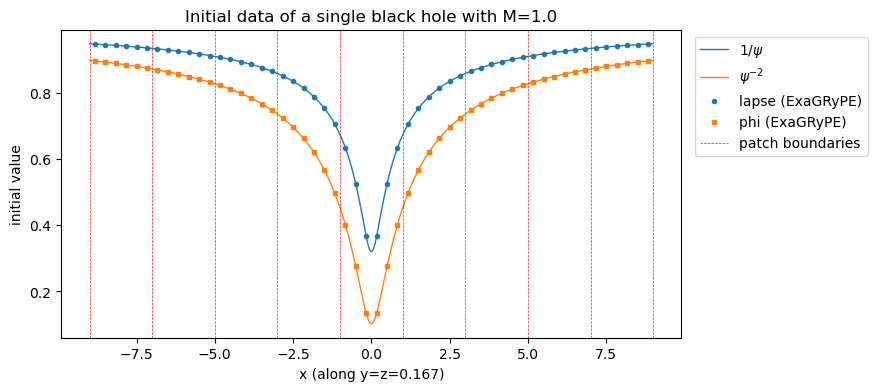
The values of all 54 volumes agree with the closed formulas up to around 5e-12. TwoPunctures hence indeed gives us a Schwarzschild black hole at the origin. Both quantities drop towards zero at the puncture, where \( \psi\) diverges. Even the volumes next to the puncture are fine, as their centres keep a distance of \( \sqrt{3} h/2 \approx 0.29\) from it. The dashed lines are the boundaries of the patches.
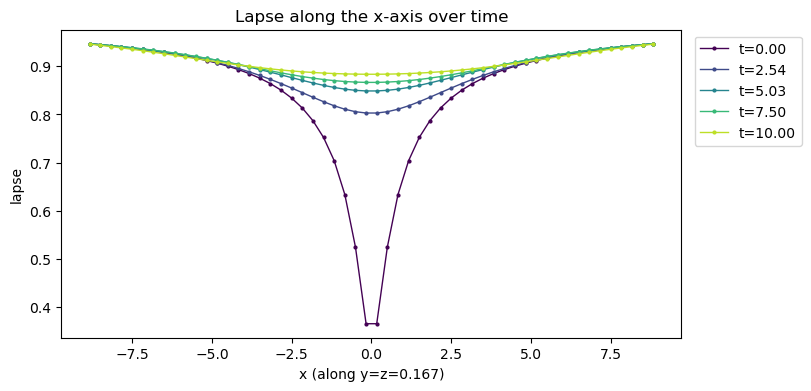
We now look at the lapse over time. First, along the x-axis for a few snapshots:
and then over time at a few distances from the puncture:
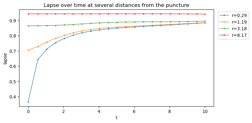
The run is stable: there are no oscillations and no NaNs, and far away from the black hole, the lapse hardly changes. Close to the puncture, however, the solution does not behave like a resolved black hole. With harmonic slicing, we would expect the lapse to collapse towards zero inside the horizon, such that the evolution freezes there. Instead, the dip of the lapse fills up. At the volume next to the puncture, the lapse grows from 0.37 to 0.88 by \( t=10\) , and the profile along the x-axis flattens out. The conformal factor phi behaves the same way: Next to the puncture, it grows from 0.13 to 0.93, i.e. almost to its value at the boundary of the domain.
The most likely reason is the resolution in combination with the scheme. The horizon has a radius of 0.5, i.e. it spans about three volumes. The Rusanov flux is first order, and, as we saw for the gauge wave, it adds a lot of numerical diffusion on coarse meshes. Here, it diffuses the steep profiles around the puncture away, and the black hole dissolves numerically. The boundary conditions, which reflect everything that travels outward, add to this. We check below that the missing constraint enforcement does not.
This is the baseline which we have to improve upon. A resolved black hole requires a much finer mesh around the puncture, which codes typically obtain by refining the mesh adaptively towards the black hole. A regular mesh of such a resolution is prohibitively expensive, which is why adaptive mesh refinement is a key extension of this setup.
So far, our run is effectively serial: Without load balancing, Peano keeps the whole mesh in one tree, and only one thread traverses it. Before we refine the mesh, we hence make the code use several cores.
Domain decomposition with an off-the-shelf heuristic explains how Peano splits the mesh into several trees, and how a load balancing strategy decides on these splits. We use the same off-the-shelf heuristic, which splits the mesh once its construction has stagnated, such that each thread gets one tree: project.set_load_balancing( "toolbox::loadbalancing::strategies::SpreadOutOnceGridStagnates", "new ::exahype2::LoadBalancingConfiguration()", ) At the same time, we refine the mesh. We keep the \( 9 \times 9 \times 9\) mesh cells, but use patches of \( 10 \times 10 \times 10\) volumes, i.e. we pass
patch_size = 10
to the numerical scheme and a maximum volume size of \( 1.01 \cdot 18/90\) to the grid construction. Each volume then has an edge length of \( h=0.2\) rather than \( 1/3\) , i.e. the mesh is 1.67 times finer along each axis and holds \( 90^3\) rather than \( 54^3\) volumes. The patch size remains even, so the puncture still sits on a vertex, and the closest volume centres keep a distance of \( \sqrt{3} h/2 \approx 0.17\) from it. A finer mesh requires smaller time steps, too, i.e. we pay twice: for more volumes and for more time steps.
We constrain OpenMP to four threads, i.e. the load balancing creates four trees:
!cd 522_single-black-hole && OMP_NUM_THREADS=4 ./single-black-hole
The log shows the split: SpreadOutOnceGridStagnates cuts the 729 mesh cells into four trees with around 182 cells each. The run now needs 338 instead of 203 time steps, and each time step takes 3.4 instead of 2.1 seconds, although it updates 4.6 times as many volumes. The whole run takes around 20 minutes on our laptop. Per volume update, the wall clock time drops from \( 13.1\,\mu s\) to \( 4.7\,\mu s\) , i.e. by a factor of 2.8. This factor is not a pure parallel speedup: Besides the four trees, the bigger patches give each patch update more volumes to work on.
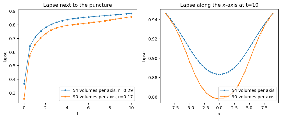
The finer mesh helps a little, but it does not change the picture. The volume next to the puncture now sits at \( r=0.17\) rather than \( 0.29\) , so its initial lapse is lower, i.e. 0.26 rather than 0.37. Yet, it fills up again, to 0.86 by \( t=10\) . Along the x-axis, the dip at \( t=10\) is slightly deeper than on the coarse mesh, 0.86 rather than 0.88, but the profile still flattens out. The horizon now spans 2.5 volumes per radius, which is still far from resolving it.
This might be the right point to tune the code further. You could
We stick to the mesh of the previous section, i.e. to \( 90^3\) volumes which four threads process, and now alter the physics rather than the performance.
The CCZ4 formulation carries algebraic constraints: The conformal metric has to have unit determinant, and the conformal extrinsic curvature has to be trace-free. The exact solution obeys them, but the numerical solution drifts away. ExaGRyPE can push the solution back onto the constraint surface after every time step via exagrype::ccz4::enforceCCZ4constraints().
exagrype.api.CCZ4Solver does not do this by default. You switch the enforcement on via enforce_ccz4_constraint(), which accepts one of three values of exagrype.api.CCZ4Solver.EnforceCCZ4Constraint:
We add solver.enforce_ccz4_constraint(exagrype.api.CCZ4Solver.EnforceCCZ4Constraint.OnlyFinalSolution) The solver then inserts an additional step after each solution update of the numerical scheme. It uses the mechanism which Additional solver steps: postprocessing the solution after each update introduces. The task graph of the time step gets an additional task "CCZ4_Enforce CCZ4 constraints after Update cell", which applies the enforcement to each volume of the patch before the solution is projected onto the faces. If you run the lowering with TEXT logging, the output lists this task. The solver knows the numerical schemes of ExaHyPE and where they write their solution. For any other scheme, it refuses to enforce the constraints and raises an exception.
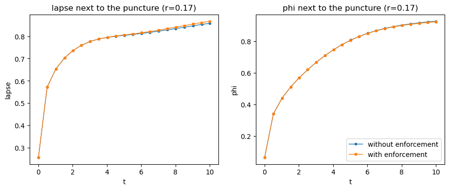
The enforcement hardly changes the outcome: Next to the puncture, the lapse grows from 0.26 to 0.87 rather than 0.86, and phi from 0.07 to 0.92 rather than 0.93. Along the whole x-axis, the lapse differs by at most 9e-3 from the run without enforcement. The additional step does not cost measurable time either: the run takes around 1100 seconds, which is within the variation of our measurements. The dissolution of the black hole hence stems from the resolution and the scheme, not from a drift away from the constraints.
So far, we hold the boundary at the initial data, i.e. everything that travels outward is reflected back into the domain. Sommerfeld conditions, also called radiative or outgoing boundary conditions, avoid most of these reflections. They assume that, close to the boundary, each field \( u\) behaves like an outgoing spherical wave which decays towards its value \( u_\infty\) at infinity:
\begin{eqnarray*} u(r,t) = u_\infty + \frac{f(r - v t)}{r}, \end{eqnarray*}
with \( v\) the speed at which the field propagates and \( r\) the distance from the centre of the domain. Differentiating this ansatz yields a condition which the boundary has to satisfy,
\begin{eqnarray*} \partial_t u + v \frac{x_i}{r} \partial_i u + v \frac{u - u_\infty}{r} = 0, \end{eqnarray*}
i.e. the solution in the ghost volumes follows from the solution inside the domain. This is the reason why our Dirichlet term cannot realise them: It sees neither the interior solution nor the normal of the boundary face.
exahype2.api therefore offers a separate PDE term, exahype2.api.SommerfeldBoundaryConditions, which you add instead of the Dirichlet term. You specify the far-field solution \( u_\infty\) and the origin, while the wave speed \( v\) is the maximum eigenvalue of your solver. There is no separate boundary task in this case: The ghost volumes are advanced whenever the face data are rolled over after the projection of a new solution (exahype2::blockstructured::applySommerfeldBoundaryConditions()).
To see what we gain, we let an acoustic pressure pulse of the Euler equations leave the domain \( [-1,1]^2\) , discretised with \( 81\) grid cells per axis, and compare the largest pressure deviation \( \max |p-1|\) from the far-field state that remains at \( t=2\) , once the pulse should have left the domain. A uniform state equal to the far field has to stay exactly where it is.
| Scheme | Uniform state | Pulse, Sommerfeld | Pulse, Dirichlet |
|---|---|---|---|
| Fourth-order Finite Differences (RK4) | exact up to round-off | \( 4.9 \cdot 10^{-4}\) | \( 5.3 \cdot 10^{-2}\) |
| Finite Volumes (Rusanov) | exact | \( 9.5 \cdot 10^{-4}\) | \( 7.6 \cdot 10^{-4}\) |
| Finite Volumes with optimistic time stepping | exact | \( 9.6 \cdot 10^{-4}\) | - |
For the fourth-order Finite Differences, the Sommerfeld conditions reduce the reflections by two orders of magnitude. The Finite Volume runs do not tell the two conditions apart: With a Rusanov flux, a ghost volume which is held at the far-field state already absorbs small waves, and the first-order scheme has damped the pulse considerably before it reaches the boundary.
To clean up, delete the generated directory. If you rerun the notebook, it is re-created.
 1.9.8