 |
Peano
|
|
Peano
|
This tutorial runs the simplest standard test of numerical relativity codes with ExaGRyPE: the gauge wave. Its exact solution is known, so we can always check what the code computes. The tutorial follows the structure of A first advection problem with the Euler equations, but instead of programming the PDE ourselves, we use the CCZ4 solver which ExaGRyPE's Python API exagrype.api ships.
We run through the following steps:
Before you start, configure and build Peano as described in Configure ExaGRyPE. You need --enable-exagrype, but not GSL: the gauge wave does not need any black hole initial data.
In this tutorial, we analyse the solution after the simulation has finished by reading the plot files. Later tutorials introduce the in-situ alternatives: tracer particles which record quantities while the code runs, on-the-fly postprocessing such as the evaluation of the constraints, and black hole spacetimes. See Advanced Usage of ExaGRyPE, A single black hole with ExaGRyPE: a first (too) trivial setup and Binary Black Hole Merger.
The gauge wave is flat (Minkowski) spacetime written down in unusual coordinates. Its line element reads
\begin{eqnarray*} ds^2 = -H \, dt^2 + H \, dx^2 + dy^2 + dz^2, \qquad H(x,t) = 1 - A \sin\left( 2 \pi (x-t) \right) \end{eqnarray*}
with the amplitude \( A=0.1\) . As the spacetime is flat, nothing physical happens. The numerical code however sees a non-trivial lapse \( \alpha = \sqrt{H}\) , a non-trivial metric and extrinsic curvature, and all of them travel with speed one along the x-axis. We simulate the unit cube with periodic boundary conditions. After \( t=1\) , the wave has crossed the domain once and is back at its initial position. The exact lapse is
\begin{eqnarray*} \alpha(x,t) = \sqrt{ 1 - A \sin\left( 2 \pi (x-t) \right) }. \end{eqnarray*}
The gauge wave is one of the standard testbeds for numerical relativity codes. The setup and the equations are discussed in Alcubierre et al.: Toward standard testbeds for numerical relativity, section IV.B. As we know the exact solution, any change of the wave's shape or amplitude is due to numerical effects.
The Python API of Peano, ExaHyPE and ExaGRyPE resides within the src directory of your Peano installation. Unless you have installed it via pip install -e ., we add it to the search path manually. We also memorise the Peano root directory, as the generated Makefile has to link against Peano's libraries.
ExaGRyPE solves the Einstein equations in the first-order CCZ4 formulation. In this formulation, the spacetime is described by 59 unknowns per point: the conformal metric \( \tilde{\gamma}_{ij}\) (six entries, as it is symmetric), the traceless conformal extrinsic curvature \( \tilde{A}_{ij}\) , the Z4 variables \( \Theta\) and \( \hat{\Gamma}^i\) , the lapse \( \alpha\) , the shift \( \beta^i\) and the auxiliary variable \( b^i\) of the gamma driver, the trace \( K\) of the extrinsic curvature and the conformal factor \( \phi\) . Since we use a first-order formulation, the spatial derivatives of lapse, shift, conformal metric and conformal factor become unknowns of their own. exagrype.api names all of them:
The lapse is unknown 16. The plotter writes these names into the output files, so we can later refer to the lapse by its name.
Every ExaHyPE 2 code starts with a project. The project describes the C++ namespace of the generated code, the name of the executable, and the directory into which all of the generated code goes. We use a subdirectory 521_gauge-wave, as the generator produces quite a lot of files and directories.
In the Euler tutorial, we created a generic exahype2.api.Solver and added the PDE terms one by one. ExaGRyPE does this for us: exagrype.api.CCZ4Solver is an exahype2.api.Solver with the 59 unknowns and all PDE terms of CCZ4 (non-conservative product, source and maximum eigenvalue) pre-registered. The terms call the kernels from the ExaGRyPE library, i.e. we do not have to write any C++ code. We only pick the initial condition. The module exagrype.api.initialvalues offers a couple of analytical setups.
CCZ4 has a number of parameters, e.g. the damping coefficients \( \kappa_1\) , \( \kappa_2\) and \( \kappa_3\) (CCZ4k1, CCZ4k2, CCZ4k3) of the constraint violations. The solver comes along with the defaults of ExaGRyPE's production runs. You can change them through the constructor's parameters argument, e.g. parameters={"CCZ4k1": 0.0}. For the gauge wave, we stick to the defaults:
We discretise CCZ4 with Finite Volumes, exactly as the Euler equations before: Each cell of the Peano mesh carries a patch of \( 9 \times 9 \times 9\) volumes. The scheme uses a Rusanov flux between neighbouring volumes and explicit Euler in time, i.e. it is a first-order scheme. The time step size follows from the CFL condition with the largest eigenvalue of CCZ4.
For the mesh, we use a regular grid. Three sizes are involved: the size of one mesh cell, the size of one volume, and the maximum volume size volume_size which we hand over to the grid construction. Every mesh cell hosts one patch, i.e. a cell's edge length is the patch size times the edge length \( h\) of one volume. Peano refines every cell as long as its edge length is greater than or equal to volume_size times the patch size. As Peano splits each cell into \( 3 \times 3 \times 3\) cells whenever it refines, a maximum volume size of 0.04 yields \( 3 \times 3 \times 3\) cells of edge length \( 1/3\) , i.e. 27 volumes per axis with a volume size of \( h=1/27\) .
The volume size \( h\) is hence always strictly smaller than the maximum volume size. Be careful if you pass in exactly the volume size that you want to obtain: A maximum volume size of \( 1/27\) asks for cells which are strictly smaller than \( 9 \cdot 1/27 = 1/3\) . Peano refines once more, and you end up with 81 volumes per axis and a code which is 81 times more expensive. Pick a maximum volume size which is slightly bigger than the volume size you want.
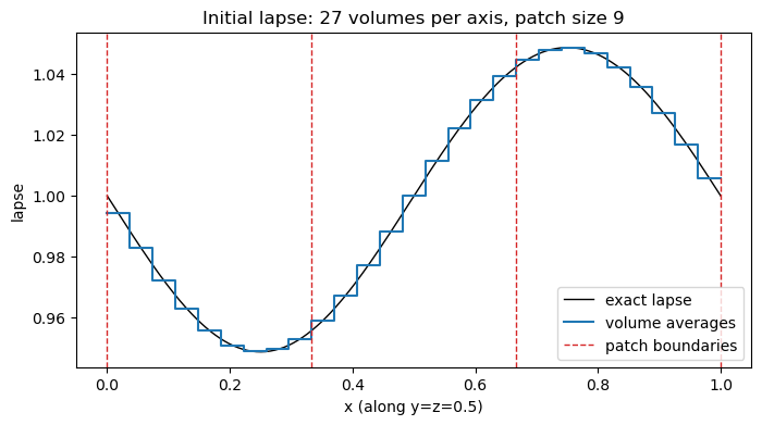
The picture below shows the initial lapse along the line \( y=z=0.5\) . The black line is the exact lapse, the blue steps are the volume averages which the Finite Volume scheme stores. The dashed red lines are the patch boundaries: Three patches with nine volumes each cover the x-axis. We sample the wave with 27 volumes per wavelength.
A three-dimensional simulation with 59 unknowns produces a lot of data. One snapshot of our coarse mesh holds \( 27^3 \cdot 59 \approx 1.2\) million values. On a mesh with 81 volumes per axis, it is 27 times more. As the gauge wave travels along the x-axis only, we do not need all of these data: We add a plot filter which restricts the output to all patches overlapping a thin box around the line \( y=z=0.5\) . The plotter then writes one row of patches only.
We also increase the plotter's precision. By default, it writes five digits. This is enough to look at the solution, but it would limit the accuracy of our convergence study later on. We plot every 0.05 time units.
We add the solver to the project and specify the domain, the time span we simulate, and the boundary conditions. We simulate exactly one period of the wave, i.e. until \( t=1\) . CCZ4 is three-dimensional only: The generated solver refuses to compile for any other dimension.
Now we lower the ExaHyPE project into a Peano project, and the Peano project into C++ code plus a Makefile. ExaHyPE has to know where Peano is installed, as the Makefile links against Peano's libraries. We pass an absolute path, as the generated Makefile resides in the subdirectory 521_gauge-wave. We also pick the release mode.
Let's see what we got:
Compared to the Euler tutorial, there is one difference: There is no solver class CCZ4.cpp for us to fill. All PDE terms are implemented in AbstractCCZ4.cpp, which delegates to the ExaGRyPE library:
As in the Euler tutorial, we tell the executable which log messages we are interested in:
We compile with make and run the executable. The code runs for around 180 time steps. On an eight-core workstation, the run takes around 25 seconds, and it writes 21 snapshots.
In the Euler tutorial, we called Peano's probe script probe.py to extract the solution at one point over all snapshots. The script is a thin wrapper around the Python class tarch.plotter.api.output.PointProbe. We can use this class directly within our notebook: We create a probe object for the point of interest, and its display() routine writes the values of all unknowns at this point over all snapshots into a csv file. There is no interpolation: The probe takes the value of the volume which contains the point. The csv file holds one row per snapshot: the time stamp followed by all unknowns, named as discussed above.
We wrap everything into a small helper routine which returns the time stamps and the lapse. The probe is chatty, so we silence its output:
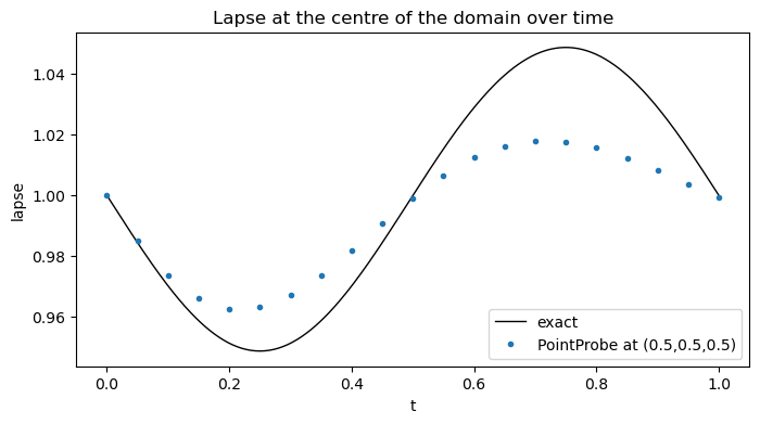
We probe the centre of the domain. The exact lapse there is \( \alpha(0.5,t) = \sqrt{1 - 0.1 \sin(2\pi(0.5-t))}\) . Please note that the code does not hit the plot time stamps exactly: It plots after the first time step which passes the next plot time stamp. We therefore compare against the exact solution at the time stamps stored in the csv file.
You should get the following picture: The observer at the centre sees the wave passing by once. The numerical solution has the right period, but it loses amplitude over time.
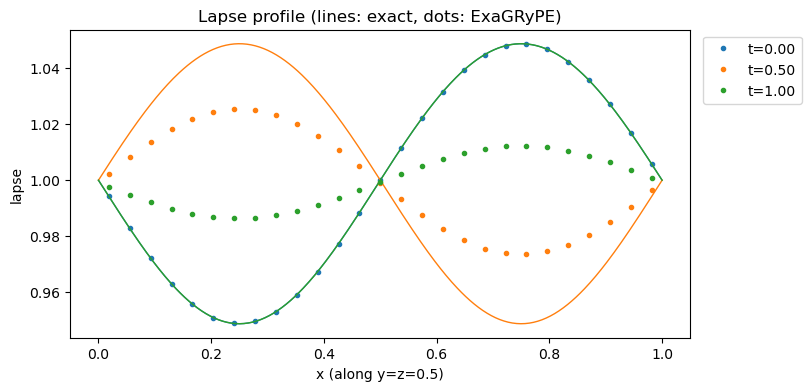
The probe gives us the time series at one point. To get the shape of the wave at one point in time, we place one probe into the centre of every volume along the line \( y=z=0.5\) . Each probe returns the whole time series, so we obtain the wave profile for all snapshots at once. With 27 volumes, this takes a few seconds.
The picture shows the lapse at \( t=0\) , \( t=0.5\) and \( t=1\) . The lines are the exact solution, the dots are the values computed by ExaGRyPE. The wave travels at the right speed: After half a period, it has moved by half the domain, and at \( t=1\) it is back at its initial position. However, the scheme smears out the peaks. This is numerical diffusion. The Rusanov flux adds artificial viscosity to keep the scheme stable, and the coarser the mesh, the stronger this effect. After one period, the amplitude has dropped from 0.05 to around 0.013, and the maximum error of the lapse is 0.038.
If you prefer to look at the solution in ParaView, convert the patch files into VTU files with Peano's render script. It relies on the ParaView/VTK Python libraries. See Visualization of ExaGRyPE Output for some remarks on the visualisation of ExaGRyPE's output. cd 521_gauge-wave python3 ../../../../src/tarch/plotter/api/render.py solution-CCZ4.peano-patch-file
The gauge wave is a convergence test: We check that the numerical error shrinks as expected when we refine the mesh. We measure the error of the lapse after one period along the line \( y=z=0.5\) ,
\begin{eqnarray*} e(h) = \max_i \left| \alpha_i - \alpha(x_i,t) \right|, \end{eqnarray*}
where \( \alpha_i\) is the value of volume \( i\) with centre \( x_i\) and \( t \approx 1\) the time stamp of the last snapshot. If we make the volumes three times smaller, the error of a scheme of order \( p\) should go down by a factor of \( 3^p\) . We hence estimate the order from two subsequent meshes via
\begin{eqnarray*} p \approx \frac{\log \left( e(3h) / e(h) \right)}{\log 3}. \end{eqnarray*}
Here, \( h\) is the volume size, i.e. the edge length of one volume, which is one over the number of volumes per axis. With patches, there are two knobs to obtain a certain volume size \( h\) : the patch size and the number of mesh cells. 27 volumes per axis result from \( 9 \times 9 \times 9\) cells with patches of size 3, or from \( 3 \times 3 \times 3\) cells with patches of size 9. Peano always refines the root cell at least once, i.e. there are at least three cells per axis. A patch size of 27 hence requires at least 81 volumes per axis. We study all combinations of the volume sizes \( 1/9\) , \( 1/27\) and \( 1/81\) with the patch sizes 3, 9 and 27 that fit to this constraint. To do so, we wrap all the steps from above into one routine which builds and runs the gauge wave in its own directory and returns the runtime:
Again, we pick maximum volume sizes which are slightly bigger than the volume sizes \( 1/9\) , \( 1/27\) and \( 1/81\) that we want to obtain. The runs with 9 and 27 volumes per axis take seconds. The runs with 81 volumes per axis take around 25 to 55 minutes each on an eight-core workstation, as they have 27 times more volumes and need three times more time steps than the runs on the coarse mesh. They are therefore switched off by default:
We get the following errors after one period. The estimated order refers to the next coarser mesh with the same patch size:
| volumes per axis | patch size | cells per axis | max error at t=1 | order | runtime |
|---|---|---|---|---|---|
| 9 | 3 | 3 | 4.84e-2 | 2 s | |
| 27 | 3 | 9 | 3.76e-2 | 0.23 | 82 s |
| 81 | 3 | 27 | 1.88e-2 | 0.63 | 53 min |
| 27 | 9 | 3 | 3.76e-2 | 23 s | |
| 81 | 9 | 9 | 1.88e-2 | 0.63 | 26 min |
| 81 | 27 | 3 | 1.88e-2 | 31 min |
Two observations stand out.
First, the patch size does not change the solution at all. For a given volume size, all patch sizes yield exactly the same error. This is what we expect: The Finite Volume scheme applies the same stencil to every volume, and the patches only determine how Peano organises the volumes in memory and how it distributes the work. The patch size does however change the runtime. With patches of size 3, there are \( 27^3\) cells on the finest mesh. Each cell comes with some administrative overhead, and each patch has to exchange a halo of one volume with its neighbours, which is expensive relative to the tiny patch. With patches of size 27, there are only 27 cells, i.e. there is little parallelism for the eight cores. Patches of size 9 are the sweet spot here.
Second, the estimated orders at \( t=1\) are well below one, although the scheme is first order. The table below shows the maximum error of the runs with patch size 3 at several points in time:
| t | h=1/9 | h=1/27 | h=1/81 | order (1/9 to 1/27) | order (1/27 to 1/81) |
|---|---|---|---|---|---|
| 0.05 | 9.32e-3 | 3.39e-3 | 1.18e-3 | 0.92 | 0.96 |
| 0.1 | 1.57e-2 | 6.59e-3 | 2.34e-3 | 0.79 | 0.94 |
| 0.2 | 2.58e-2 | 1.21e-2 | 4.57e-3 | 0.69 | 0.89 |
| 0.5 | 4.21e-2 | 2.48e-2 | 1.05e-2 | 0.48 | 0.78 |
| 1.0 | 4.84e-2 | 3.76e-2 | 1.88e-2 | 0.23 | 0.63 |
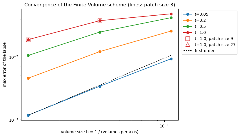
Early on, the error indeed shrinks by a factor of three whenever we make the volumes three times smaller. Over time, the numerical diffusion damps the wave away. The error cannot grow beyond the amplitude of the wave, which is 0.05. On the coarsest mesh, the wave has almost entirely disappeared after one period, i.e. the error has saturated. Such a mesh is not in the asymptotic regime where the error behaves like \( h^p\) , and the order estimates drop. The picture shows the maximum error over the volume size for the four points in time. The lines are the runs with patch size 3. The squares and triangles show that the runs with patch sizes 9 and 27 sit exactly on top of them.
If you want to measure a convergence order, you hence either have to stop early or to refine further until all meshes are in the asymptotic regime. The latter quickly becomes expensive: A run with 243 volumes per axis would need around 81 times as long as a run with 81 volumes per axis.
Exercise:** Compute the convergence order for the L2 error along the line instead of the maximum error, and compare the error of the lapse with the error of another unknown such as the trace of the extrinsic curvature (traceK). The analytical solution of all unknowns is implemented in exagrype::initialvalues::gaugeWave() in src/exagrype/initialvalues/InitialValues.cpp.
The pictures of this tutorial are created by the script tutorials/exahype2/exagrype/illustrations/521_gauge-wave.py, which runs exactly this study.
Our setup has a few limitations which you should be aware of:
solver.numerical_scheme  = exahype2.api.rkfd4.CentralDifferencesWithRungeKutta(solver, patch_size, rk_order=4)
solver.grid_construction = exahype2.api.rkfd4.SetupSimulationOverRegularGrid(solver, volume_size=max_volume_size)
solver.plotter           = exahype2.api.rkfd4.PlotAsVTKFile(solver, first_plot_time_stamp=0.0, time_in_between_plots=0.05, plotter_precision=10)
On our mesh with 27 grid cells per axis, the maximum error of the lapse after one period (t=1) drops from roughly 4e-2 with Finite Volumes to roughly 5e-5 with fourth-order Finite Differences. Unlike the legacy ExaGRyPE, exahype2.api.rkfd4 supports regular grids only so far.
To clean up, delete the generated directories. If you rerun the notebook, they are all re-created.
 1.9.8