ExaHyPE's prime parallelisation strategy is the domain decomposition of Peano. Peano enumerates all cells of the mesh along a space-filling curve, cuts the resulting sequence of cells into chunks, and makes each chunk a subdomain of its own. Technically, each subdomain is a tree of its own, i.e. a part of the overall spacetree.
Peano uses these trees both for MPI and for multithreading: The trees are distributed among the ranks, and each rank then processes its local trees in parallel. Even a pure OpenMP code therefore relies on the domain decomposition. If the mesh is not split up, all cells form one big tree, and there is little work for the other threads to grab. ExaHyPE can add tasking on top of this, but the domain decomposition remains the baseline.
Peano itself never decides when and how to split up the mesh. This decision is made by a load balancing strategy. Without any load balancing, ExaHyPE installs toolbox::loadbalancing::strategies::NoLoadBalancing, i.e. the mesh remains one tree. In this tutorial, we
- take the Euler solver from A first advection problem with the Euler equations and add load balancing to it,
- discuss what happens throughout the setup of the simulation once a load balancing is in place, and
- visualise the resulting subdomains with ParaView.
ExaHyPE's domain decomposition page collects further background information.
Prerequisites
The domain decomposition only pays off if Peano has been configured with multithreading and/or MPI support, e.g. by adding
--with-multithreading=omp --with-mpi=mpicxx
to the configure call, where you pass your MPI compiler wrapper to –with-mpi. Invoke ./configure –help to see which options are on the table. With CMake, use the corresponding WITH_MULTITHREADING and WITH_MPI options. After that, you have to rebuild Peano. All ExaHyPE applications then pick up these settings. This tutorial runs with multithreading only, so you do not need MPI.
The solver
We use the same Euler solver as in A first advection problem with the Euler equations, with patches of \( 9 \times 9\) Finite Volumes on a regular mesh over a periodic domain:
import sys, os
sys.path.insert(0, os.path.abspath("../../src"))
import exahype2
namespace = ["tutorials", "exahype2", "domaindecomposition"],
project_name = "Euler",
directory = "30_domain-decomposition",
executable = "euler",
)
patch_size = 9
"EulerFV",
4,
0,
)
solver,
first_plot_time_stamp = 0.0,
time_in_between_plots = 0.01,
)
project.add_solver(solver)
project.set_global_simulation_parameters(
dimensions = 2,
offset = [-0.1, -0.1],
size = [0.2, 0.2],
min_end_time = 0.02,
max_end_time = 0.02,
periodic_BC = [True, True, True],
)
The conservative flux F(Q) of a hyperbolic PDE.
Point-wise initial condition: given the physical position of a single degree of freedom,...
The maximum absolute eigenvalue of the flux Jacobian in a given direction, i.e.
Abstract base class for all ExaHyPE 2 solvers.
Plotting counterpart to RusanovWithExplicitEuler: maps the patch data of a Finite Volume scheme with ...
Finite Volumes with a Rusanov Riemann solver and explicit Euler time stepping, realised over a block-...
Setup phase counterpart to RusanovWithExplicitEuler: sets the initial condition for a Finite Volume s...
Adding load balancing
Load balancing is added by one line. We pass the fully qualified name of the load balancing strategy plus the arguments of its constructor:
project.set_load_balancing(
"toolbox::loadbalancing::strategies::SpreadOutOnceGridStagnates",
"new ::exahype2::LoadBalancingConfiguration()",
)
toolbox::loadbalancing::strategies::SpreadOutOnceGridStagnates waits until the mesh construction has stagnated, i.e. until the grid statistics report that the most recent mesh sweep has not refined the mesh any further. It then splits up the mesh in one rush, such that each thread on each rank gets one tree. After that, it does not split anymore.
The second argument is handed over to the strategy's constructor. Here, it is an instance of exahype2::LoadBalancingConfiguration, which constrains the splits. Its constructor accepts, in this order,
- the load balancing quality, i.e. the ratio between the lightest and the heaviest rank which we accept as good enough (default 0.9);
- the minimum number of cells per tree. Smaller trees are not split up any further (default 0, i.e. no constraint);
- whether we assume periodic boundary conditions (default false, see the discussion of the decomposition below);
- the maximum number of trees per rank throughout the initial distribution (default: one per thread);
- the maximum number of trees per rank afterwards (default: two per thread);
- the split mode, i.e. whether we split bottom-up or top-down (default bottom-up).
Picking the arguments is a trade-off: The more trees and the better the balancing, the more expensive the decomposition becomes, as each split temporarily requires additional memory and mesh sweeps. Studying a few settings for a particular experiment hence is worth the effort.
Tailoring the configuration
We stick to the default configuration in this tutorial. Two examples of tailored configurations read as follows. The first one asks for a balanced bottom-up splitting, where no tree is smaller than 512 cells, and it allows up to twice as many trees as threads after the initial distribution:
project.set_load_balancing(
"toolbox::loadbalancing::strategies::SpreadOutOnceGridStagnates",
"new ::exahype2::LoadBalancingConfiguration("
"0.95, " # load balancing quality
"512, " # minimum size of a tree (cells)
"false, " # assume periodic boundary conditions
"::exahype2::LoadBalancingConfiguration::UseNumberOfThreads, " # max trees throughout initial distribution
"::exahype2::LoadBalancingConfiguration::UseTwiceTheNumberOfThreads, " # max trees afterwards
"peano4::SplitInstruction::Mode::BottomUp" # split mode
")"
)
The second one splits more aggressively top-down into smaller trees, but it caps the number of trees at two throughout the initial distribution and at four afterwards:
project.set_load_balancing(
"toolbox::loadbalancing::strategies::SpreadOutOnceGridStagnates",
"new ::exahype2::LoadBalancingConfiguration("
"0.98, " # load balancing quality
"256, " # minimum size of a tree (cells)
"true, " # assume periodic boundary conditions
"2, " # max trees throughout initial distribution
"4, " # max trees afterwards
"peano4::SplitInstruction::Mode::AggressiveTopDown" # split mode
")"
)
SpreadOutOnceGridStagnates is only one of several built-in strategies. The overview of the load balancing strategies lists them, and the load balancing toolbox explains how they work. You can obviously also write your own strategy: Implement a subclass of toolbox::loadbalancing::AbstractLoadBalancing, pass its fully qualified name to set_load_balancing(), and make it available to the build. The generated main file includes the header whose path matches the class name, i.e. a strategy mylb::MyStrategy has to be declared in mylb/MyStrategy.h.
We can now generate the code:
project.set_Peano4_installation(os.path.abspath("../../"), peano4.api.output.CompileMode.RELEASE)
peano4_project = project.generate_Peano4_project()
peano4_project.generate()
What happens throughout the setup
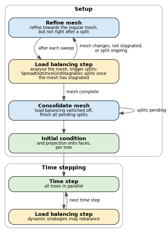
The setup phase with load balancing, followed by the time stepping
The load balancing interacts with the setup phase of the simulation, which exahype2.api.fv.SetupSimulationOverRegularGrid builds:
- Refine mesh. The setup repeats this mesh sweep while the mesh still changes, while the load balancing has not yet stagnated, or while a split is still being carried out. After each sweep, the load balancing gets the opportunity to analyse the mesh and to trigger splits. Splits are expensive, so the sweep does not refine any further right after a split. Otherwise, the freshly split trees would immediately become unbalanced again.
- Consolidate mesh. Once the mesh has been constructed, the setup switches the load balancing off and keeps on running mesh sweeps until the mesh is stationary and all splits have been carried out.
- Initial condition and projection onto faces. These steps run on the final decomposition, i.e. each tree initialises its own cells.
The time stepping then informs the load balancing after each time step, too. SpreadOutOnceGridStagnates has already done its job at this point, but strategies which rebalance dynamically use these notifications.
Building and running the code
We take the implementation of EulerFV from the Euler tutorial:
%%writefile 30_domain-decomposition/EulerFV.cpp
void tutorials::exahype2::domaindecomposition::EulerFV::flux(
const double* __restrict__ Q, const tarch::la::Vector<Dimensions, double>& x, int normal, double* __restrict__ F
) {
const double irho = 1.0 / Q[0];
constexpr double gamma = 1.4;
const double p = (gamma - 1.0) * (Q[3] - 0.5 * irho * (Q[1] * Q[1] + Q[2] * Q[2]));
switch (normal) {
case 0:
F[0] = Q[1];
F[1] = irho * Q[1] * Q[1] + p;
F[2] = irho * Q[1] * Q[2];
F[3] = irho * Q[1] * (Q[3] + p);
break;
case 1:
F[0] = Q[2];
F[1] = irho * Q[2] * Q[1];
F[2] = irho * Q[2] * Q[2] + p;
F[3] = irho * Q[2] * (Q[3] + p);
break;
}
}
void tutorials::exahype2::domaindecomposition::EulerFV::maxEigenvalue(
const double* __restrict__ Q, const tarch::la::Vector<Dimensions, double>& x, int normal, double* __restrict__ lambdaMax
) {
const double irho = 1.0 / Q[0];
constexpr double gamma = 1.4;
const double p = (gamma - 1.0) * (Q[3] - 0.5 * irho * (Q[1] * Q[1] + Q[2] * Q[2]));
const double c = std::sqrt(gamma * p * irho);
// velocity, i.e. momentum divided by density
const double u = Q[1 + normal] * irho;
lambdaMax[0] = std::max(std::abs(u + c), std::abs(u - c));
}
void tutorials::exahype2::domaindecomposition::EulerFV::initPointWisely(
const tarch::la::Vector<Dimensions, double>& x, double* __restrict__ Q
) {
// One period of a sine density profile over the periodic domain
// [-0.1,0.1], constant velocity u and constant pressure p
constexpr double gamma = 1.4;
constexpr double p = 1.0;
constexpr double u = 1.0;
const double rho = 1.0 + 0.2 * std::sin(2.0 * M_PI * (x[0] + 0.1) / 0.2);
Q[0] = rho;
Q[1] = rho * u;
Q[2] = 0.0;
Q[3] = p / (gamma - 1) + 0.5 * rho * u * u;
}
The number of trees SpreadOutOnceGridStagnates creates depends on the number of threads. With OpenMP, we set the thread count through the environment, and we run the code with four threads:
!cd 30_domain-decomposition && make -j > make.log 2>&1 && OMP_NUM_THREADS=4 ./euler > run.log 2>&1 && echo done
The load balancing reports the trees after each mesh sweep. The final report lists four trees. Their numbers of local cells, i.e. the first number per tree, add up to the 729 cells of the mesh:
!grep "dumpStatistics" 30_domain-decomposition/run.log | tail -1
Each tree writes its own patch file per snapshot, and the file solution-EulerFV.peano-patch-file stitches them together. The subdomain a patch belongs to is hence preserved in the output.
Visualising the subdomains with ParaView
To study the decomposition in ParaView, we convert the patch files into VTU files with Peano's render script:
!cd 30_domain-decomposition && PYTHONPATH=../../../src python3 ../../../src/tarch/plotter/api/render.py solution-EulerFV.peano-patch-file > render.log 2>&1 && echo done
Open the resulting solution-EulerFV.EulerFVQ.pvd in ParaView and press Apply. The array "Unknowns (EulerFVQ, subdomain)" holds the four unknowns of the Euler equations, followed by the number of the subdomain that a patch belongs to. Colour by this array and pick its last component, i.e. component 4. Next, open the colour map editor, tick "Interpret Values As Categories", and pick a qualitative colour map such as "Brewer Qualitative Set2". Each subdomain then gets a colour of its own:
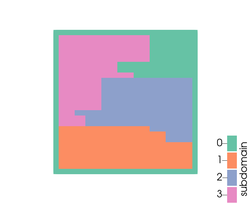
The subdomains of the Euler run with four threads in ParaView
The mesh is split into four subdomains with around 182 cells each, i.e. one per thread. The subdomain number is the position of a tree's patch file within the snapshot. It hence does not necessarily coincide with the tree number from the log.
The subdomain which hosts a frame along the whole domain boundary is tree 0, i.e. the tree the other trees have been split off from. This is not a coincidence: We use periodic boundary conditions, and Peano realises them as a data exchange of tree 0 with itself. Therefore, cells adjacent to a periodic boundary are never given away to another tree (see peano4::grid::Spacetree::isCellSplitCandidate()). Tree 0 keeps all of them, and the load balancing assigns tree 0 fewer interior cells instead. If you use periodic boundary conditions with many ranks, set the argument assumePeriodicBoundaryConditions of exahype2::LoadBalancingConfiguration to true. The configuration then imposes a minimum tree size throughout the initial distribution, which leaves tree 0 enough cells to hold the boundary.
Where to go from here
- If Peano is configured with MPI, you run the code with mpirun, e.g.
mpirun -np 2 ./euler. The very same load balancing then distributes the trees among the ranks first and among the threads per rank afterwards.
- SpreadOutOnceGridStagnates is a good starting point, but it splits only once. The strategy overview discusses the alternatives, and the load balancing API provides Python tools to analyse and postprocess the decompositions.
- The offline load balancing tutorial shows how to compute a decomposition once and to feed it into subsequent runs.

 1.9.8