 |
Peano
|
|
Peano
|
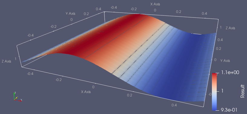
The Peano plotting will be automatically switched on if users pass a positive args.plot_step_size. The code will then try to plot at every given step size in code time, and it will plot the initial snapshot and the final snapshot when args.end_time is reached, even if it just dumps a regular snapshot according to the time interval. The default plotting format of Peano is the patch file, which contains the solution arrays in each cell; each thread on each rank will dump its own patch file in a parallel run.
The following commands convert the Peano patch files into standard vtu files, which can then be inspected in other standard visualization tools such as ParaView.
The render script supports parallel snapshot processing, and you can set the number of processes you would like to run at the same time by setting the parameter after -j.
In the Python API script of ExaGRyPE, users are allowed to control the clips/parts and the variables they would like to have in their snapshot files. There are lines like
If you set project.add_plot_filter as \( ([a,b,c],[d,e,f], K)\), the code will dump all patches that contain cells having coordinates within the rectangular clip \( ([a,b,c], [a+d,b+e,c+f]) \). The final parameter indicates the frequency of the plotting (plot when the \( K \)th time the plot_step_size is reached; 1 is recommended). In the example code above, a slice of the x-y plane will be output. By specifying select_dofs_to_print, users can control the size of the solution array per cell. In ExaGRyPE, we have 58 basic variables plus extra monitoring variables; the basic variable mapping is given below:
\( [0]\tilde{\gamma}_{xx},[1]\tilde{\gamma}_{xy},[2]\tilde{\gamma}_{xz},[3]\tilde{\gamma}_{yy},[4]\tilde{\gamma}_{yz},[5]\tilde{\gamma}_{zz},\\ [6]\tilde{A}_{xx},[7]\tilde{A}_{xy},[8]\tilde{A}_{xz},[9]\tilde{A}_{yy},[10]\tilde{A}_{yz},[11]\tilde{A}_{zz},\\ [12]\Theta,[13]\hat{\Gamma}^x,[14]\hat{\Gamma}^y,[15]\hat{\Gamma}^z,\\ [16]\alpha,[17]\beta^x,[18]\beta^y,[19]\beta^z,[20]b^x,[21]b^y,[22]b^z,\\ [23]A_x,[24]A_y,[25]A_z,\\ [26]B^x_x,[27]B^y_x,[28]B^z_x,[29]B^x_y,[30]B^y_y,[31]B^z_y,[32]B^x_z,[33]B^y_z,[34]B^z_z,\\ [35]D_{xxx},[36]D_{xxy},[37]D_{xxz},[38]D_{xyy},[39]D_{xyz},[40]D_{xzz},\\ [41]D_{yxx},[42]D_{yxy},[43]D_{yxz},[44]D_{yyy},[45]D_{yyz},[46]D_{yzz},\\ [47]D_{zxx},[48]D_{zxy},[49]D_{zxz},[50]D_{zyy},[51]D_{zyz},[52]D_{zzz},\\ [53]K,[54]\phi,[55]P_x,[56]P_y,[57]P_z. \)
Here we provide a brief introduction on how to inspect the output files, using a snapshot from a single black hole simulation as an example. The converted vtu file can be opened directly in ParaView:
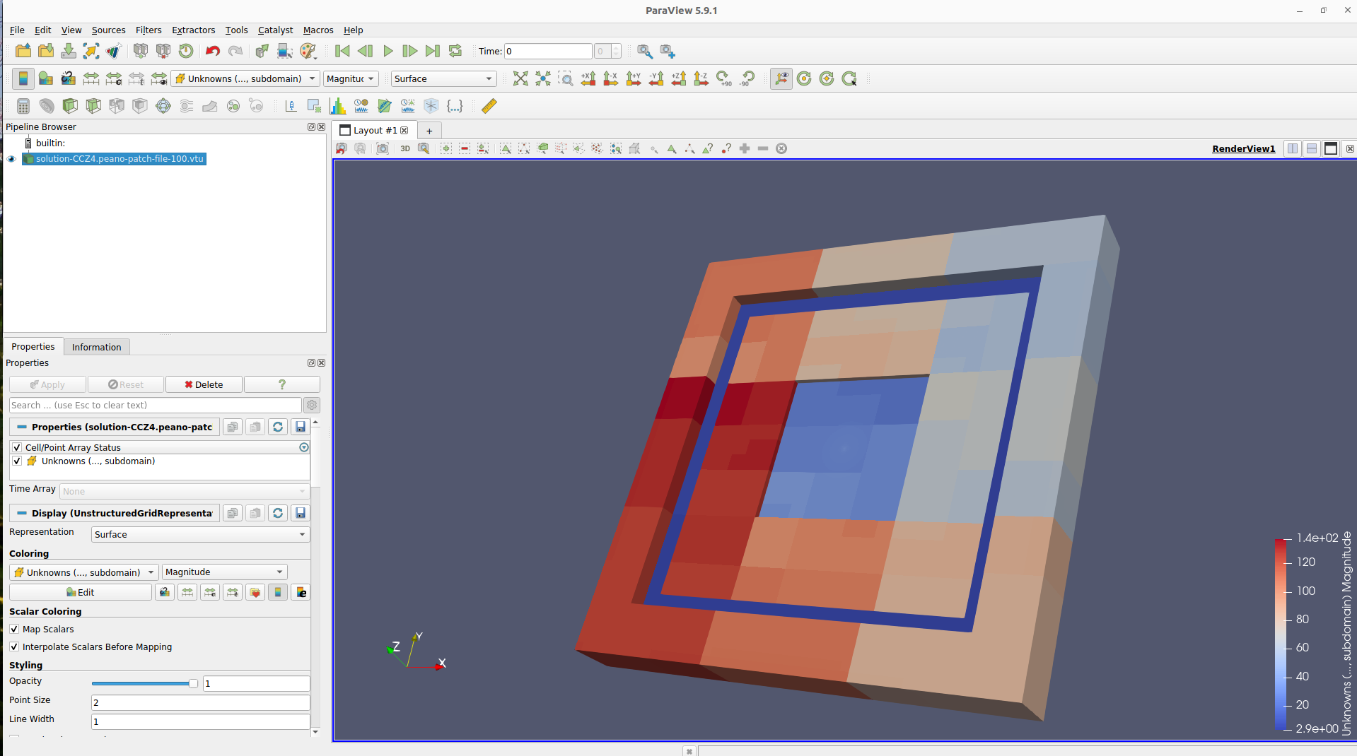
As the patch sizes differ across different AMR levels, the thickness differs accordingly. Using the slice tool (fourth in the third line of the quick toolbars) and choosing Z normal gives you an actual slice of the x-y plane of the simulation. You can also switch to "surface with edges" from "surface" on the second line of the quick toolbars to check the AMR pattern:
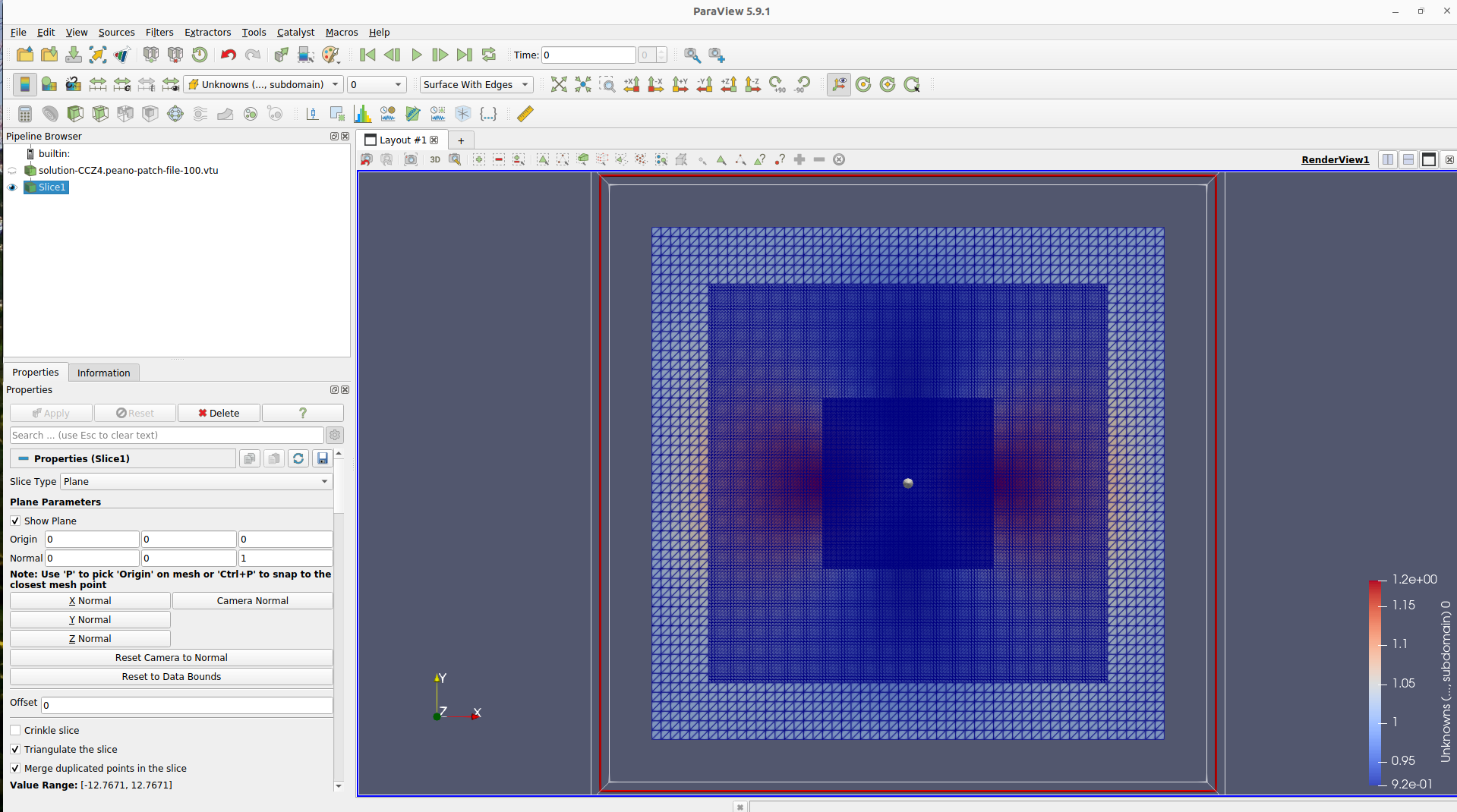
Using the list in the second line of the quick toolbar you can select the variables you would like to inspect. For black hole spacetimes, the most characteristic variables one may look into are the conformal factor ( \( \phi \), 54), the lapse function ( \( \alpha \), 16), and the physical constraints ( \( H, M_i \), 59-62 if outputted). Using the plot over line tool, you can check the profiles of variables in a separate panel:
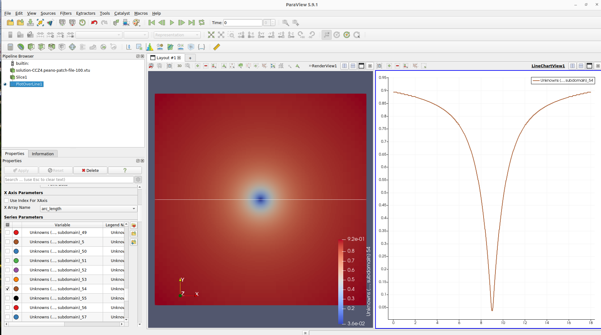
You can switch among snapshots of different timestamps using the buttons on the first line of the quick toolbars. For the Single Schwarzschild Black Hole, the solution should remain static after some relaxation time. Therefore, the colour map and the profiles of the variables should change only little, if at all, in the snapshots from the later stages of the simulation.
 1.9.8