This documentation is autogenerated from ./tutorials/exahype2/hpc/gpus.ipynb. Once you clone the Peano repository, please work against this notebook or study Peano's generic description how to generate web docu from Jupyter notebooks.

Prepare the setup

We assume that you have configured your code with multithreading by adding

--with-multithreading=Pick

to the configure script. Invoke the automake script with –help to see what options are on the table. In CMake, all configuration works analogously. After that, you have rebuild your whole code. Once complete, all ExaHyPE 2 applications will pick up these settings for their code, i.e. we can continue to execute this notebook.

If you want to profile or optimise your code further, you might want to pick a particular vendor toolchain. See configure's help on --with-toolchain. The logging section discusses variations of the toolchain support.

Configuring the environment

The first thing we will do is importing the Peano 4 and ExaHyPE 2 API. While we could do this in the terminal via export PYTHONPATH=$PYTHONPATH:$PEANO_ROOT/python, We again work directly within the notebook. Once on the Python path, the core packages can be imported just like any other package:

import sys, os
 
sys.path.insert(0, os.path.abspath("../../../python/"))
 
import peano4.api, exahype2

If some of these imports fail due to missing packages, either install through your preferred system environment or install them straightaway from within the notebook (this is not the elegant version, as you might spot/derive from the –break-system-packages attribute):

import sys

!{sys.executable} -m pip install --break-system-packages scipy mpmath sympy

Demo solver

To make the tutorial do something, we pick one of our simplest exercise solvers, create an ExaHyPE 2 project, and add this solver to the project:

exahype2_project = exahype2.Project(
    namespace=["tutorials", "exahype2", "exercises", "acoustic"],
    project_name="Acoustic",
    directory=".",
    executable="exahype2-acoustic"
)

dimensions = 2
patch_size = 16
cell_h = 1.1 * 2.0 / (3.0 ** 3)
 
my_solver = exahype2.solvers.fv.rusanov.GlobalFixedTimeStep(
    name                  = "PlanarAcousticSolver",
    patch_size            = patch_size,
    min_volume_h          = cell_h/patch_size,
    max_volume_h          = cell_h/patch_size,
    normalised_time_step_size = 0.01,
    unknowns              = 3,
    auxiliary_variables   = 0
)

All the implementation is ready to go in the tutorials section. Nothing here is special - we simply follow the (solutions of the) exercises.

my_solver.set_implementation(
    flux = exahype2.solvers.PDETerms.User_Defined_Implementation
)

The ExaHyPE 2 project:

The solver setup is not in any way surprising either:

!mkdir solutions

exahype2_project.add_solver(my_solver)

exahype2_project.set_output_path("solutions")

exahype2_project.set_global_simulation_parameters(
    dimensions            = 2,
    size                  = [2.0,  2.0],
    offset                = [-1.0, -1.0],
    min_end_time          = 1.414,  # sqrt(2)
    max_end_time          = 1.414,  # sqrt(2)
    first_plot_time_stamp = 0.0,
    time_in_between_plots = 0.1,
    periodic_BC           = [True, True],
)

Activate GPU offloading

By default, ExaHyPE uses the task orchestration that we have introduced with our IWOMP paper (see the generated README-xxx.md file once the Python script has terminated). You can alter this scheme by

project.set_load_balancing( "tarch::multicore::orchestration::Hardcoded::createNative()" )

for example, which replaces Peano's bespoke tasking back-end with a native back-end where literally each and every task are directly mapped onto a TBB, OpenMP, SYCL or C++ task.

Now we kick the lowering off:

exahype2_project.set_Peano4_installation("../../../", peano4.api.output.CompileMode.Release)
peano4_project = exahype2_project.generate_Peano4_project()
peano4_project.generate()

Adding the actual Physics

So far, we have created a framework for a solver, but we have not written anything actually. We only told ExaHyPE that there will be a user-defined solver one day. So let's see what we actually got from the code so far:

!ls *.cpp *.h

ExaHyPE/Peano have given us a couple of files:

There is the main file plus its header. This is kind of the driver of our simulation. We can alter it, but often the default does the job.
There is the Constants.h which holds all the global simulation parameter that we've specified before.
The AbstractPlanarAcousticSolver class is an implementation of our numerical scheme of choice and the baseline of our actual solver.
Its implementation PlanarAcousticSolver then holds the actual physics. Let's have a look into this one:

!cat PlanarAcousticSolver.h

!cat PlanarAcousticSolver.cpp

You can obviously study the superclass, as well. But for our purpose the only important thing is that are four functions that we have to befill. Actually, we can ignore the boundary implementation, as we have picked periodic BCs, i.e. they won't be called anyway. This leaves us with the flux and the eigenvalue and the initial condition.

Our development workflow from hereon is clear:

We write those functions.
We build the code (that's a plain make as Peano gives us a good old Makefile)
We run the simulation

Exercise: Implement the flux and eigenvalue

Open the cpp file of your implementation and add in the realisation of the flux and the eigenvalue. The formulae can be found above. The eigenvalue is always the same independent of any parameters and returns a scalar as per function signature. The flux is either first column or the second column from the matrix above, depending on the value of normal. For the initial condition, let's use a very simple hard-coded one for the time being:

 void ::exahype2::...::initialCondition(
   [[maybe_unused]] const double* __restrict__                   Q, // Q[3+0]
   ...
 ) {
   const double val = cos(-tarch::la::PI*(volumeCentre[0] + volumeCentre[1]));
   const double K0 = 4.0, rho = 1.0;
   const double kr = std::sqrt(2 * K0 * rho);
   Q[1] = val;
   Q[2] = val;
   Q[0] = kr * val;  // that's the p
 }

It might be more elegant to move rho and K0 as static consts into the header of the solver, but this does the job. Next, compile and execute:

!make -j

!./exahype2-acoustic

Visualisation

Finally, once the program has finished running, we can convert the output from the native peano4 format into something that can be visualised.

Peano 4 provides a script for this, which can be called via python3 $PEANO_ROOT/python/peano4/visualisation/render.py followed by the name of the files we want to convert.

This relies on the ParaView/VTK Python libraries, and converts the files into .vtu files, which can be visualised for example using ParaView.

import subprocess
render_environment = os.environ.copy()
render_environment["PYTHONPATH"] = f"../../../python:{render_environment['PYTHONPATH']}"
 
!{sys.executable} -m pip install --break-system-packages vtk
 
 
subprocess.call(
    ["python3", "../../../python/peano4/visualisation/render.py", "solutions/solution-PlanarAcousticSolver.peano-patch-file"],
    env=render_environment
)

Initial conditions

Solution

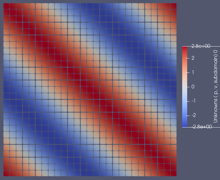
The solution is rather straightforward: double exahype2::...maxEigenvalue( ... ) { const double K0 = 4.0; const double rho = 1.0; const double c = std::sqrt(4.0 / rho);

return c; }

 void ::exahype2::...::flux(
  ...
 ) {
   const double K0 = 4.0, rho = 1.0;

   switch(normal) {
     case 0: // Flux in x-direction
       F[0]  = K0 * Q[1];
       F[1]  = Q[0] / rho;
       F[2]  = 0.0;
       break;
     case 1: // Flux in y-direction
       F[0]  = K0 * Q[2];
       F[1]  = 0.0;
       F[2]  = Q[0] / rho;
   }
 }