 |
Peano
|
|
Peano
|
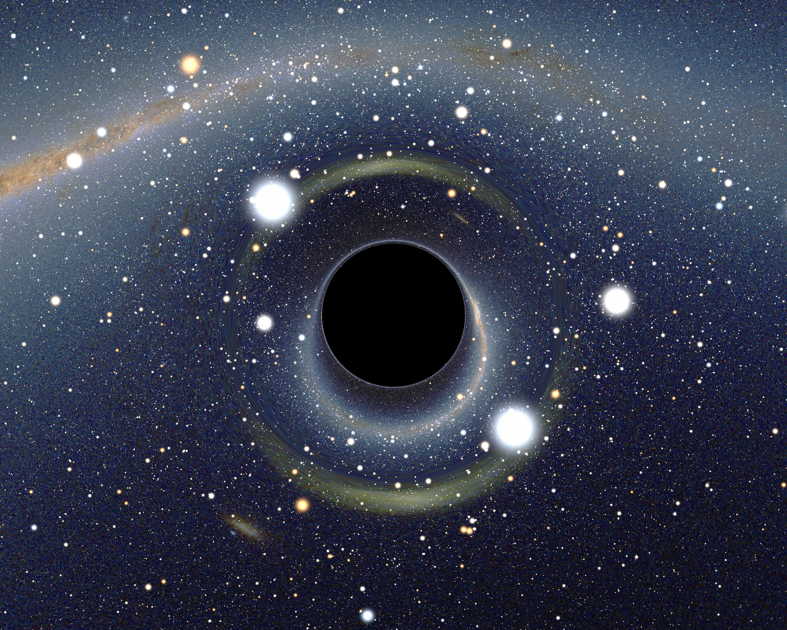
Illustration from Wikimedia Commons shared under Creative Commons Attribution-Share Alike 2.5 Generic license.
This benchmark solves the single black hole (Schwarzschild black hole) with ExaGRyPE.
To understand what is going on here, it might help to read through ExaGRyPE first. According to the description there, ExaGRyPE solves a wave equation, i.e. it models how the effects of mass ripple through spacetime.
In this benchmark, however, we solve for a stationary black hole. Such an object does not really exist (real black holes rotate, accrete matter, and therefore grow), but it provides a good test case for our numerical methods, not least because plenty of reference data and analytical solutions are available.
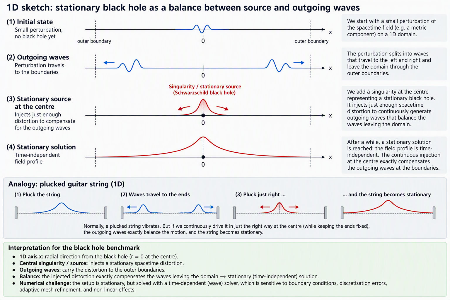
At the centre of the simulation domain, we have a singularity, i.e. a right-hand-side term that represents a stationary distortion of spacetime. It is chosen such that it injects just enough change into spacetime at the centre to counteract the waves travelling out through the boundary of the simulation domain.
You can think of this as similar to a guitar string that we pluck in the middle while holding it tight. Normally, the string would vibrate, but here we pluck it in just the right way to counteract the vibration, so everything becomes stationary.
While the output is not particularly exciting (the simulation should eventually yield a stationary solution), the problem is numerically challenging. Boundary-condition effects, discretisation errors, adaptive mesh refinement effects, and other numerical artefacts all feed into a strongly nonlinear equation system that can easily blow up and become unstable. Solving a stationary setup with a time-dependent solver is therefore an excellent stress test.
The single black hole benchmark needs some time to burn in and reach a stationary state. After that, we have to evolve it long enough to be reasonably confident that there are no tiny little wiggles in the outcome that eventually could blow up. Indeed, sometimes we have small errors that travel towards the domain boundary. If they are not properly absorbed there, they can reflect back into the domain. As they travel forth and back and we inject more and more error, the simulation blows up. So we have to evolve the whole setup long enough. We go beyond what most papers do at ask for t=100.
If we pick the domain too small, we will almost certainly mess up the boundary conditions. This setup employs Sommerfeld conditions, which are designed to absorb outgoing waves and should not reflect them back into the domain. However, they are only an approximation, and they are only valid if the waves are far enough away from the boundary. There will always be some reflection, and the smaller the domain, the stronger the reflection. So we pick a \( [486,486,486]^3 \) domain offset by \( [-243,-243,-243] \) so its centre is at the origin, which is where the singularity (black hole) is located.
The maximum mesh size is a mesh spacing (volume size) of
volume_size = 0.4
for Finite Difference and Finite Volume schemes. For DG, you can allow a mesh size of 4.0, but at least fourth-order spatial resolution is needed.
As it is a stationary setup, we don't know what time stepping scheme is mandatory. One would at least expect the order to match the spatial order (so usually 4th order Runge-Kutta), but maybe a lower order scheme is sufficient. As starting point, we recommend to use the same time stepping scheme as in the gauge wave benchmark, i.e. 4th order Runge-Kutta.
Sommerfeld boundary conditions are used, which are designed to absorb outgoing waves and should not reflect them back into the domain. Besides these boundary conditions, you might have to use Kreiss-Oliger dissipation if you employ a fourth order scheme.
The settings below resemble content discussed in A single black hole with ExaGRyPE: a first (too) trivial setup. It makes sense to run through this tutorial and the tutorials before that one, before you start benchmarking the single black hole setup as discussed here.
For this single black hole benchmark, the following Peano toolboxes are mandatory:
--enable-blockstructured)--enable-exahype, this switches on ExaHyPE 2)--enable-exagrype)In theory, the benchmark passes without parallelisation. In practice, it is so computationally demanding that we recommend to use multithreading and MPI. Due to this, you also need
--enable-loadbalancing)GPU support is, as always, optional. Other advanced features such as particle tracers are not used. However, you will need GSL. GSL is trivial to enable
--with-gsl
but depending on your system, you might have to load the GSL module separately before you build (and run) the application:
GSL's headers and library have to be found by the compiler (gsl-config --version has to work). If you configure Peano without GSL (see benchmarks_exagrype_single_black_hole_configure), the code generator still works, but the compiler stops with the message "exagrype.api.initialvalues.single_black_hole() requires TwoPunctures: configure Peano with --with-gsl". The initial data comes from TwoPunctures, which is only part of the ExaGRyPE library if GSL was enabled.
The benchmark uses the Autotools build (the CMake build works with the analogous ENABLE_*/WITH_* options). The following line is what the measurements below used (Intel oneAPI 2024.2 icpx, OpenMP, an 8-core workstation):
Some remarks:
--enable-exahype --enable-blockstructured --enable-loadbalancing --enable-exagrype --with-gsl are mandatory, see above. --enable-particles is not needed.-g does not slow down the code, but it is required if you want to profile with line information.--with-multithreading=omp is what the thread counts of the performance study refer to (OMP_NUM_THREADS). The performance study only makes sense with multithreading. There is also a oneTBB version of the code, a native C++ version and a sycl version.-I<vtune>/include to the compiler flags and -L<vtune>/lib64 to the linker flags and LIBS=-littnotify. The profiles below did not rely on the API: they use VTune's software sampling and need nothing more than -g._debug, _asserts, _strace, _stats). The build variants of the benchmark pick them: debug links _debug, profile links _stats and production links the plain release libraries. Make sure make has completed without errors before you start: all three variants of the benchmark need the libraries of ExaHyPE 2 and ExaGRyPE in the flavour you use (src/exahype2/libExaHyPE2Core3d*.a, src/exagrype/libExaGRyPECore3d*.a).requirements.txt: pip install -e . in a virtual environment, or export PYTHONPATH=<peano>/src.make there. Add --peano-directory <path to Peano> to single-black-hole.py if the script is not run from within benchmarks/exagrype/single-black-hole (the studies script does this for you).A first test whether everything works:
builds in about 20 s and finishes after about 4 s on eight cores.
All experiments are driven by single-black-hole.py. It generates, builds and (together with studies-single-black-hole.py) runs the setup. The script does not write checkpoints by default, and the studies below do not need them.
The parameters above (domain 486, volume size 0.4, t=100) describe a run with more than three billion volumes. This is impossible on a workstation. The script therefore distinguishes three variants through --variant:
| Variant | Compile mode | Domain | Volume size | End time | Purpose |
|---|---|---|---|---|---|
| debug | Peano debug build | 18 | 1.2 | 0.5 | Does the code work at all? |
| profile | Peano stats build | 54 | 1.2 | 5 | Small enough to profile and to run parameter studies on one node. |
| production | Peano release build | 486 | 0.4 | 100 | The setup from above. |
The variant fixes the defaults of --domain-size, --volume-size and --end-time. You can override each of them explicitly. Unless you study the numerics of the full domain, work against the profile variant.
The maximum mesh size of the README is a hard bound: the mesh must never be coarser than the regular mesh with --volume-size. Adaptive mesh refinement (AMR) therefore does not coarsen the far field. It refines the regular mesh further around the black hole, where the singularity sits and the solution varies strongest:
python3 single-black-hole.py --scheme fv --amr-levels 1 --amr-radius 4 --variant profile
adds one level (factor three, i.e. volumes three times smaller per axis) to every cell within distance 4 of the puncture. The criterion depends on the position only and never asks for an erase; the mesh is static. As the time step size of the explicit schemes scales with the smallest volume, one level makes the time step three times smaller.
min mesh size=..., #local cells=...). Take them into account when you choose --amr-levels: one level costs a factor of 14 (radius 1), 25 (radius 4, one thread) or 40 (default radius 12, eight threads) in runtime on the profile mesh, two levels did not fit into the 15 GB of our workstation (11 GB with a single thread, and hours of runtime). The default radius of 12 refines a block that is far too big for the profile variant. Use --amr-radius 1 or 4 there. The script studies-single-black-hole.py with the argument schemes builds and runs
| Name | Scheme |
|---|---|
| fv-regular, fv-amr-1 | Finite Volumes (Rusanov, explicit Euler) on the regular mesh and with one additional level (radius 1) |
| fd4-rk2, fd4-rk3, fd4-rk4 | Fourth-order Finite Differences with Runge-Kutta of order 2, 3 and 4 |
| fd4-rk4-lopsided | fd4-rk4 plus lop-sided advection along the shift |
| fd4-rk4-lopsided-ko | fd4-rk4-lopsided plus Kreiss-Oliger dissipation (sigma=8) |
Each configuration is built into its own subdirectory; the results land in studies-schemes/results-schemes.csv (exit code and wall time per run) next to the console log of every run. As the README explains, the stationary solution is a stress test: a scheme that is not stable ends with a non-zero exit code or aborts early.
The directory slurm-scripts holds examples for a cluster with Slurm (the module names follow Hamilton at Durham; adapt the partitions, the modules and the path to your Peano checkout through PEANO):
| Script | Purpose |
|---|---|
| schemes.slm | The scheme study on one node. |
| performance-array.slm | The performance study as an array job, one task per thread count (sbatch uses the task ID as thread count). |
| production.slm | The production setup with AMR on several nodes with MPI. Build before you submit. |
 1.9.8
