Load Balancing (Domain Decomposition)

Table of Contents

• Usage through Python API
• Overview over some pre-manufactured load balancing strategies
• Implementation remarks
  • Load balancing variations
  • Rebalancing, joins and AMR
• Visualising and understanding the domain decomposition
  • Displaying the domain decomposition in Paraview
  • Visualising Tree structure with spliting
  • Performance flaws
• Tuning and Tailoring the domain decomposition
  • Load balancing throughout mesh construction
  • Domain decomposition for existing partitions or late throughout the mesh construction
• Formalisation of load balancing

Suite of generic load balancing algorithms (strategies) for Peano 4.

The toolbox::loadbalancing::strategies namespace hosts various primitive strategies, but you can combine them into more sophisticated cascade of load balancing schemes. You find examples for such cascades in the namespace toolbox::loadbalancing::strategies::cascade.

All these strategies have one simple purpose: They have to invoke peano4::parallel::SpacetreeSet::split() at the right point. That is, Peano does not offer any built-in load balancing. In principle, it requires the user code to call split() at one point and hence to trigger the domain decomposition. In some codes, the split can be found in the main routine of the simulation. However, if each and every user writes their own load balancing, we quickly end up with redundant data.

Therefore, this toolbox provides some generic load balancing schemes. Still, you have to add calls to this toolbox to your main, and the toolbox might benefit if you feed in additional settings and information. At the end of the day, the workflow however remains the same:

• You tell Peano to run through the mesh.
• Every now and then, you invoke the load balancing toolbox which might, hidden away from you, trigger rebalancing.
• You continue to invoke mesh traversals, and these will then somehow realise additional splits (as well as joins).

Usage through Python API

Many extensions, such as ExaHyPE 2, not only use the load balancing toolbox, they also offer a tailored ExaHyPE 2 load balancing configuration, i.e. they provide means for users to employ the toolbox without interfering with the main functions or calling the load balancing manually. Indeed,the toolbox follows the philosophy that the chosen load balancing determines the load balancing strategy, while the configuration object tailors this strategy to your experimental setup and machine.

• See more on how to configure load balancing within ExaHyPE 2.
• There's a dedicated page on the parallelisation aspects within ExaParty.

Overview over some pre-manufactured load balancing strategies

• toolbox::loadbalancing::strategies::Hardcoded Don't do any analysis but hand out the partitioning instructions following a rulebook. This version allows you to create a reproducible load balancing scheme or to manually determine the splitting.
  Offline helpers (see Load balancing API) yield an enumerated list of splits, i.e. four lists splittingTrees, numberOfCells, subTrees (subtree ids) and bottomUpFlags, where entry k describes the kth split. The strategy itself decides when to issue the kth split. Interpretation:
  • splittingTrees = unique parent subtree id for all introduced cells of the split, or 0 if ambiguous.
  • numberOfCells = number of cells that switch ownership across a parent–child edge (child is target subtree, parent exists and has a different subtree id). For level 0, it is the number of cells on level 0 that already belong to the target subtree.
  • subTrees = subtree identifiers (not MPI ranks); you must map them to destinationRanks for the Hardcoded constructor.
  • bottomUpFlags = whether the split is a bottom-up or top-down split.
• toolbox::loadbalancing::strategies::SpreadOut Ensure that, if the problem is large enough, each thread on each rank gets one partition.
• toolbox::loadbalancing::strategies::SpreadOutHierarchically This strategy is very similar to toolbox::loadbalancing::strategies::SpreadOut, but is spreads out in two phases. First, the strategy tries to give each rank a partition. From thereon, each rank tries to give each of its threads one partition.
• toolbox::loadbalancing::strategies::RecursiveBipartition As the name suggests, the load balancing tries to identify oversized partitions and then splits these guys into two.

Implementation remarks

The toolbox's strategies typically have a

• blacklist (toolbox::loadbalancing::Blacklist)
• configuration (toolbox::loadbalancing::Configuration)
• cost metrics (toolbox::loadbalancing::CostMetrics)
• state (toolbox::loadbalancing::State)
• statistics (toolbox::loadbalancing::Statistics)

These are generic properties modelled as attributes of toolbox::loadbalancing::AbstractLoadBalancing. Each attribute is in turn a class of its own. They have all different jobs. Please consult the individual class documentations for further details.

Load balancing variations

Besides "primitive" generic load balancing strategies realising one particular approach, you can also design cascades of load balancing strategies. Cascades are chains of different strategies. Whenever the Nth strategy comes to the conclusion that its load balancing has either terminated or stagnated, a cascade switches to the N+1th strategy to continue.

A lot of strategies have default settings. All the load balancing strategies work against some cost metrics metrics and the default here for example is loadbalancing::metrics::CellCount. But you can create your own cost metric and use this one instead, which might give you better balanced subdomains.

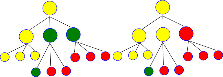
Of particular relevance is not only the decision when to split and where, but also how to split up the domain further. Peano supports two different split modes: bottom-up along the space-filling curve, and top-down within the spacetree. The latter approach is similar to recursive kd-decomposition. Each approach comes along with pros and cons. SFC-based partitioning makes it easier to have well-balanced domains, but the arising subdomain topology (who is adjacent to whom and what happens with coarser levels) can become tricky. Furthermore, you will have to know your mesh structure completely to construct good SFC subpartitions. Recursive top-down decomposition lends itself to domain decomposition which kicks in directly while we create the tree.

Not all strategies support both domain splitting schemes. You have to consult their documentation. Before you do so, I strongly recommend to read through Peano's domain decomposition remarks, and maybe even to read the paper

@article{Weinzierl:2019:Peano,
  author =       {T. Weinzierl},
  title =        {The Peano software---parallel, automaton-based, dynamically adaptive grid traversals},
  journal =      {ACM Transactions on Mathematical Software},
  year =         {2019},
  volume =       {45},
  number =       {2},
  pages =        {14}
}

which is available through the gold access route.

Rebalancing, joins and AMR

Peano does not support rebalancing with joins. That is, once a domain is split into two parts, the cuts in-between these parts will stay there forever. Almost. If a domain A splits into A and B, and if B degenerates, i.e. hosts exclusively unrefined cells, then B can be instructed to join A again.

This strict commitments to tree-like joins and forks makes the implementation easier - notably in a multiscale context. You can still oversubscribe the threads, i.e. create more logical subpartitions than threads, and hence mimic diffusion-based load balancing for example.

Dynamic AMR is no problem for the domain decomposition. That is, a refined region can ripple or propagate through a domain cut. However, Peano will never deploy a cell to another tree if that cell hosts a hanging vertex and its parent cell is not deployed to the same tree, too. This constrains notably the SFC-based bottom-up splitting. You might encounter situations where the AMR effectively "stops" the SFC decomposition from adding further cells to a new domain. The reason for this policy is that the tracking of multiscale data consistency between hanging nodes on different trees otherwise becomes unmanageable hard.

Visualising and understanding the domain decomposition

In the toolbox.loadbalancing toolbox, you find a script plot-load-distribution.py which creates plots over the data distribution. The invocation is close to trivial

python3 ~/git/Peano/src/toolbox/loadbalancing/api/postprocessing/plot_load_distribution.py mpi/ccz4-backfill-fv-0.05-4-ranks.results

though you might want to study the help dumped if you pass –help.

The script works for shared and distributed memory and gives you a scatter plot over the load distribution and tells you also how many trees aka subpartitions you employ per rank.

Displaying the domain decomposition in Paraview

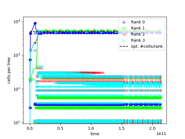
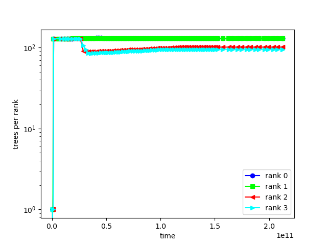
The Peano output patch files contain the information of domain decomposition for you to inspect. You can convert the patch files to standard vtu files using the postprocessing script of Peano:

pvpython ~/git/Peano/python/peano4/visualisation/render.py your_output.peano-patch-file

The vtu files can be visualised via a visualisation software, and we take Paraview as the example. In Paraview you can switch to the last variable of the grid which represents which tree the volumes belong to:

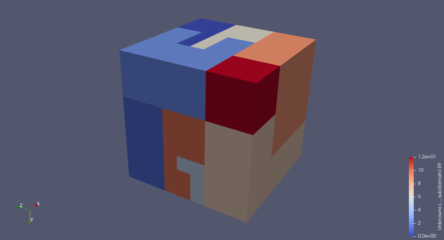
You can further look into individual trees by adding Filters - Calculator to extract the field information

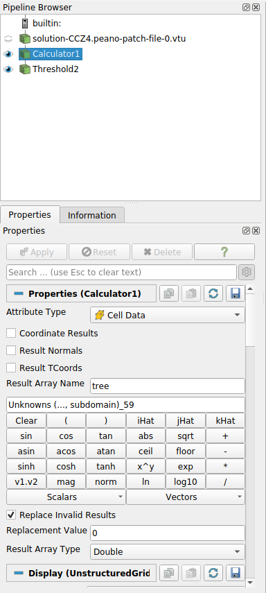
and then apply Filters - Threshold where you can alter the minimum and maximum to visualise the certain partition:

Visualising Tree structure with spliting

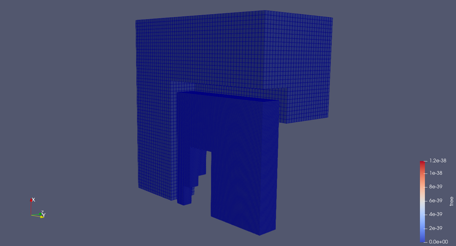
For information of the whole structure, you need to first enable the grid plot property of your solver:

MySolver.__init__(
  ...,
  plot_grid_properties=True
)

And launch a new simulation with only one snapshot output for your interested timestamp (to aviod duplicate domain info from multiple snapshot, you can use parameter of ploting start time and simulation ending time to achieve this. Obviously for static AMR the initial timesnapshot will do the work)

Then use the python script for postprocessing

pvpython ~/git/Peano/python/exahype2/postprocessing/treeReaderWithSplit.py -file-path your-grid-file-folder

it will then provide the visuilasation of the whole trees structure, with different color squres representing nodes from different subtrees. The whole tree will be illustrated so the first matrix will always be 3^d, then 9^d, 27^d,...etc.

Performance flaws

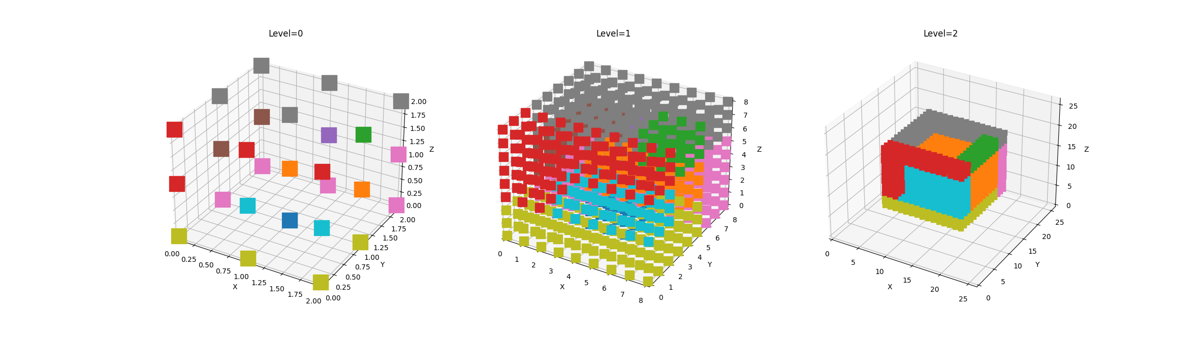
Inappropriate or problematic domain decomposition decisions will always manifest in performance flaws. There are a few further resources that discuss generic details which are not tied to this toolbox. However, they are very useful to get the most out of this toolbox:

• Peano has a dedicated runtime analysis discussion which can help to understand the runtime behaviour shaped by the domain decomposition.
• Peano has a dedicated page on performance optimisation. It discusses many flaws and how to fix them. The page below discussed more the rationale and provides background information why things work the way they do.

Further to the generic Peano discussions, individual extensions have their own specific discussion of how to analyse and to understand performance characteristics, which in turn again might relate to domain decomposition decisions:

• Peano's runtime analysis discussion and its performance optimisation recipes.
• ExaParty's performance optimisation discussion.

Tuning and Tailoring the domain decomposition

While the toolbox offers some generic load balancing schemes, it will not be able to accommodate all applications. It notably will always lack domain-specific knowledge. However, there are generic tuning knobs and considerations. The page below summarises some generic rationale and lessons learned. Particular flaws and their fixes are discussed on the Peano optimisation page. So we get an explanation of things here, why things work the way they do. The recipies how to spot flaws and how to fix them are discussed on the generic page.

Load balancing throughout mesh construction

Every load balancing strategy in Peano 4 will have to balance two contradicting objectives:

• Load balancing has to happen as soon as possible throughout the grid construction process, as we want the grid construction to run in parallel. Splits in itself are also extremely memory-demanding—at least temporarily as parts of a partition have to be replicated and moved around—so we prefer setups that perform these splits before we have a lot of mesh data in place that has to be moved around.
• Load balancing performs best if triggered for reasonably big meshes, as finer meshes allow for better tree cuts. If we know how many cells there are, we can balance these cells better, and we can subdivide cells more accurately: If we deploy a 3x3 grid to two cores, one core will get 5 and one 4 cells. If all cells refine once more, this will induce a 45 vs 36 mesh. If we cute a 9x9 mesh in a balanced way, we get a 41 vs 40 mesh. So the more we know, i.e. the closer the constructed mesh to the real final mesh, the better our domain.

The first argument is a strict one. If we run out of memory, the simulation will crash. The second argument is a desireable one.

We derive generic guidelines for any load balancing:

• Split up aggressively initially such that a reasonable initial load decomposition is achieved: There are no single partitions of extreme size left over which will eventually be split up further. Such single large partitions might make us run out of memory later on.
• Split aggressively for small partitions, split only once or twice per traversal later on when there are large partitions.
• Fine tune a load decomposition as late as possible, when accurate SFC cuts in the mesh can be made. Keep in mind that we cannot diffuse load decompositions. We can only merge with a master and then resplit.
• Throttle the grid construction or a grid refinement whenever we rebalance. Rebalancing is already problematic from a memory constraint point of view. Any further refinement makes this situation worse.
• Maybe try not to use all cores immediately. Most Peano schemes (and the default configurations) try to have a most two logical subdomains per thread. If we go beyond this, they stop further decomposition. It therefore makes sense to have a few subpartitions pre rank early on, so the mesh construction runs in parallel, but to spare some threads, i.e. to have fewer subdomains than threads, until the mesh is reasonably fine and accurate.

Domain decomposition for existing partitions or late throughout the mesh construction

It can makes sense to take into account that aggressive top-down splitting can handle AMR boundaries, while bottom-up SFC cuts struggle (see implementation). Consequently, you might want to switch between these flavours, too: SFC-based partitioning is good if a mesh is rather regular.

As soon as you have a mesh with a lot of AMR in it, it can be advantageous to switch to top-down domain decomposition. SFC-based approaches struggle to create subdomains spanning AMR boundaries (for technical reasons). The to-down approach basically does recursive kd-partitioning and hence is way more robust w.r.t. AMR.

Peano favours - due to its name - the bottom-up SFC-based decomposition, but most load balancing flavours also have a variant which uses top-down splitting. Please consult all classes within toolbox::loadbalancing::strategies.

Formalisation of load balancing

There is a dedicated subpage Load balancing strategies which describes load balancing with graph theoretic glasses on.

For offline decomposition and analysis of adaptive mesh trees, there is a dedicated subpage: Load balancing API

Postprocessing of load balancing data is a dedicated page only discussing scripts that we ship to visualise the outcomes.