 |
Peano
|
|
Peano
|
In Domain decomposition with an off-the-shelf heuristic, the load balancing decides at runtime when and how to split up the mesh. Such generic strategies work for all kinds of meshes, but they know little about the particular experiment, and they have to find out about the mesh while it is constructed.
If we know the mesh before we run the code, we can compute the decomposition ahead of time, i.e. offline, and hard-code the outcome. This is particularly simple for static meshes. Offline load balancing is a straightforward way to get a reasonable decomposition for a particular experiment, and it can serve as a baseline for something more bespoke and dynamic later on. In this tutorial, we
The load balancing strategies formalise the problem that we solve here and explain what makes a good decomposition. The load balancing API documents all the Python routines that we use below.
We use exactly the same Euler solver as in the domain decomposition tutorial. We wrap it into a function, as we will need the setup twice:
The offline load balancing works on a Python representation of the spacetree. Our mesh is regular: With patches of \( 9 \times 9\) volumes of size 0.001, each cell has to be smaller than 0.009. The spacetree hence is refined three times, i.e. the finest level holds \( 27 \times 27 = 729\) cells. We do not have to read this mesh from a file, as we can synthesise it:
Next, we split the tree. We want one subtree per thread, i.e. four subtrees. The equidistant decomposition gives each subtree the same number of cells, and split_tree() assigns the cells to the subtrees. It runs through the cells along the same space-filling curve that Peano uses when it traverses the mesh: Subtree 0 gets the first cells along the curve, then subtree 1 gets the next chunk, and so forth.
Our domain is periodic. Peano never hands over cells along a periodic boundary, i.e. these cells always stay on tree 0. We therefore pass the periodic boundary conditions to split_tree(), which keeps these cells on subtree 0 and counts them towards subtree 0's share:
Finally, we map the subtrees onto ranks and translate the outcome into the arguments of the hardcoded load balancing. As we run on one rank only, all subtrees go to rank 0. Tree 0 is the tree that all other trees are split off from, so we only need destination ranks for the other three trees. We also ask for bottom-up splits, which we discuss below:
toolbox::loadbalancing::strategies::Hardcoded takes an enumerated list of splits, i.e. three lists plus the split mode. Entry \( k\) of the lists describes the \( k\) th split:
We do not say when a split happens. The strategy hands out the splits in the order given, and it issues the \( k\) th split as soon as its splitting tree holds more than number_of_cells cells. While the mesh is constructed, tree 0 first holds 9 and then 81 cells, which is not enough. Once tree 0 holds all 729 cells, all three splits go out in one mesh sweep.
Each split comes with a mode which tells Peano how to pick the cells that it hands over:
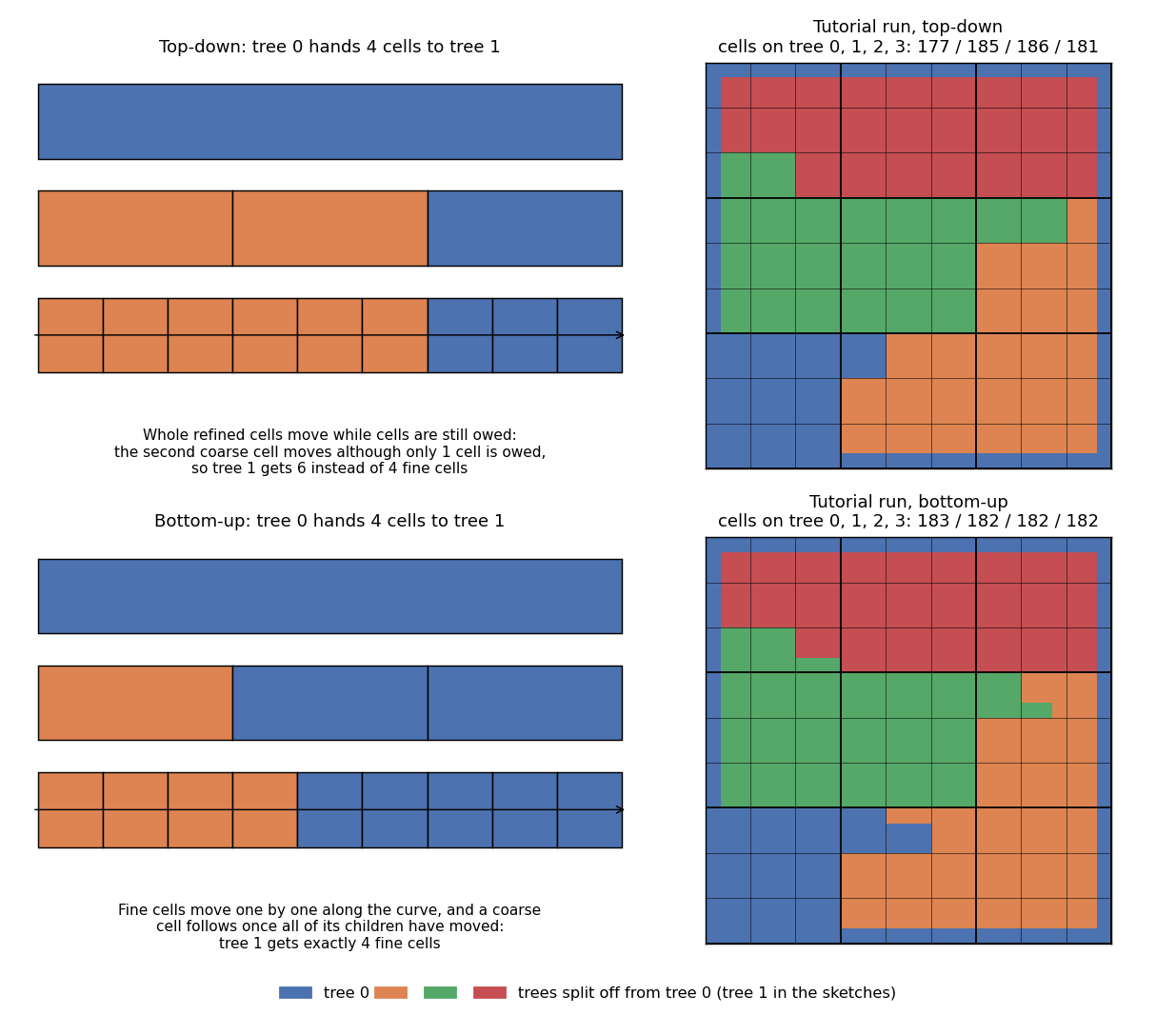
As we want Peano to reproduce our plan cell by cell, we use bottom-up splits. create_constructor_initialisation_string() accepts either a single marker Hardcoded.TopDown or Hardcoded.BottomUp, or one marker per split. Without markers, it infers the modes from the decomposition.
If you use more than one rank, pass the number of ranks as max_ranks. The constructor string is the same on all ranks, and each rank only issues the splits of the trees that it hosts. Peano's tree numbers encode the rank which hosts a tree, i.e. tree \( t\) lives on rank \( t \bmod R\) for \( R\) ranks. The subtrees of the offline plan therefore have to be assigned to the ranks round robin, as assign_trees_to_ranks_round_Robin() does. We always assume this assignment, and create_constructor_initialisation_string() checks it.
The constructor string is all that we hand over to the project:
If you prefer to write C++ yourself, e.g. within your own main, the call above corresponds to
You can also pass one mode per split instead of one mode for all splits.
The remaining steps are the same as in the domain decomposition tutorial:
The log shows how the hardcoded load balancing hands out its splits, and the final distribution of the cells among the trees:
Each tree reports two numbers, e.g. #1:182/410: The first one counts the cells that the tree owns and updates. The second one counts the virtual cells of the tree, i.e. cells that the tree knows about but that belong to others. Tree 0 additionally owns the coarse cells above the splits. Virtual cells do not do any calculation. They however have to be stored, traversed and kept consistent with the tree that owns them. Virtual cells arise where the subdomains of different trees meet: The more ragged the subdomain boundaries, the more coarse cells a tree has to know about to reach its own fine cells. We hence want to keep their number small (see also the load balancing strategies, which measure a decomposition by its imbalance and its surface).
We convert the output and open it in ParaView as described in the domain decomposition tutorial:
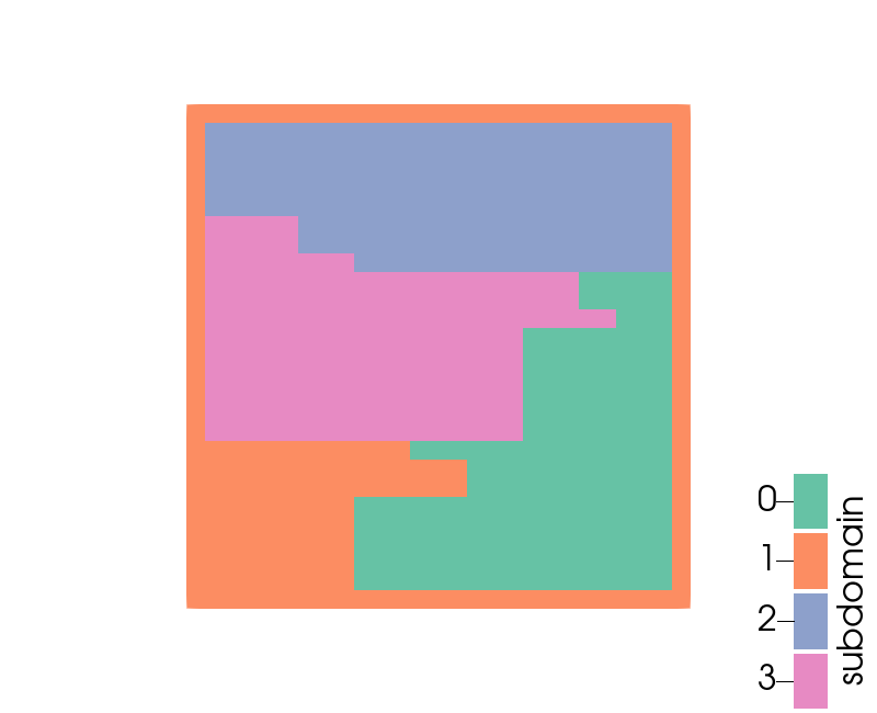
ParaView numbers the subdomains in the order in which the trees write their output files. These numbers hence need not match Peano's tree numbers: Above, the frame belongs to tree 0, even though ParaView labels it differently.
The trees hold 183, 182, 182 and 182 cells, i.e. exactly the numbers of the offline plan. Indeed, Peano builds the planned subdomains cell by cell:
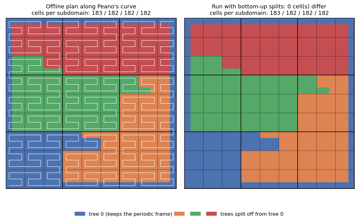
Tree 0 keeps a frame along the whole periodic boundary, plus the first cells along the space-filling curve. The other trees each get one chunk of the curve.
Two remarks are due. First, the frame belongs to tree 0 no matter what. If you split into many trees, the frame might be larger than tree 0's fair share, and the last tree then gets fewer cells. Second, Peano runs through the space-filling curve forth and back in alternating mesh sweeps. The offline load balancing ignores this: It always plans along the forward curve. If a split happens in a backward sweep, its subdomain sits at the other end of the curve, but it still gets the planned number of cells. In our example, all split-off trees request the same number of cells, so the subdomains do not change at all. It is always worth checking the actual distribution in the log.
The equidistant decomposition above gives each tree the same number of cells. In 2d, it cuts 729 cells into chunks of 183, 182, 182 and 182 cells. These numbers have nothing to do with the structure of the spacetree: Along the space-filling curve, the chunk boundaries cut through the middle of \( 3 \times 3\) patches of cells and through the middle of coarser \( 9 \times 9\) patches. Each tree then has to carry virtual copies of the coarse cells it cuts.
The quantised decomposition chooses chunk sizes that match the tree. It only hands out chunks of the sizes \( 1 \cdot 3^{kd}, 2 \cdot 3^{kd}, \ldots, (3^d-1) \cdot 3^{kd}, 1 \cdot 3^{(k+1)d}, \ldots\) cells, i.e. (multiples of) complete subtrees: With \( d=2\) , the chunk sizes are multiples of 9, and then multiples of 81. Whatever cannot be handed out within these chunk sizes is added to the share of the next tree. The last tree gets the remainder. Switching to this strategy is a one-line change in the offline load balancing, as we replace Decomposition.equidistant_splitting() by Decomposition.quantised_splitting():
The four trees now receive 162, 162, 162 and 243 cells, i.e. all chunks are multiples of 81 cells, and the chunk boundaries line up with the boundaries of \( 9 \times 9\) blocks of cells. The price is a worse balance: The largest tree holds 243 instead of 183 cells. Everything else is identical to the equidistant case, and we again split the tree, let the periodic frame stay with tree 0, and translate the outcome into a constructor string. As the chunks are complete subtrees, top-down splits (Hardcoded.TopDown) would hand over the same cells as bottom-up splits. We stick to the bottom-up splits:
We build a second project with this configuration. It lives in its own directory and reuses the solver implementation of the first run:
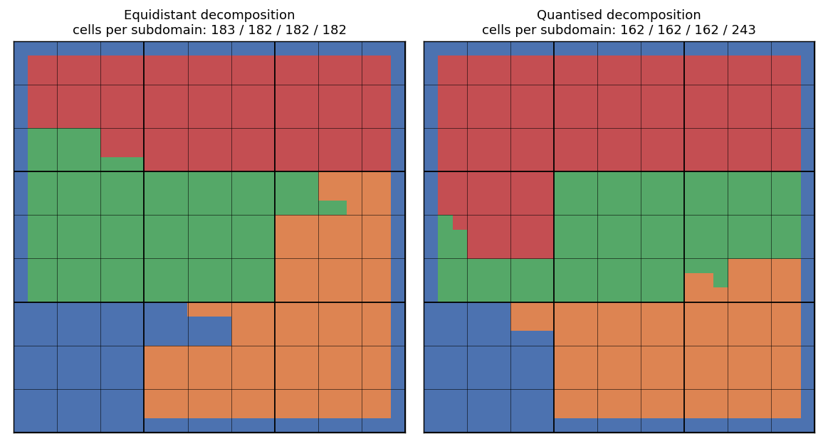
The quantised subdomains mostly consist of complete \( 9 \times 9\) blocks, whereas the equidistant subdomains end in ragged staircases everywhere. Not all raggedness vanishes: The periodic frame stays on tree 0 and takes its cells out of the blocks, so a few blocks next to the frame are still cut.
Fewer ragged edges do not automatically mean fewer virtual cells, though. Compare the totals in the last column of the output above: In this tiny example, the quantised run reports more virtual cells than the equidistant run (1123 vs. 1075). The mesh of 729 cells is so small that the periodic frame and the coarse cells that all trees share dominate the count. The quantised decomposition pays off for bigger meshes without such a frame:
Fewer virtual cells have to be bought with a worse balance, as the quantised chunk sizes fit the number of cells less well. Whether this pays off depends on how much the virtual cells cost. We have tried this on the benchmarks/exagrype/single-black-hole benchmark (Finite Volumes for the CCZ4 equations, regular mesh, eight trees on eight threads, one rank). The benchmark offers the same switch as --decomposition quantised, and studies-load-balancing.py in the same directory runs the comparison. We measure the number of virtual cells relative to the number of cells that actually compute:
| Mesh | Decomposition | Virtual cells / cells | Cells of the largest tree | Time per time step |
|---|---|---|---|---|
| 729 cells | equidistant | 5.3 | 92 | 0.189 s |
| 729 cells | quantised | 4.4 | 108 | 0.189 s |
| 19,683 cells | equidistant | 1.6 | 2461 | 3.6 s |
| 19,683 cells | quantised | 1.15 | 2916 | 3.6 s |
On these meshes without a periodic frame, the quantised decomposition removes between a fifth and a third of the virtual cells, yet the runtime does not change: The better balance of the equidistant decomposition and the smaller number of virtual cells of the quantised decomposition cancel out, or neither of them dominates the runtime. In particular, the speedup of the eight-thread run over the single-thread run stays at around 4.3 for the small mesh in either case. Virtual cells hence are not the reason why this code does not scale perfectly on a node. Measure before you pay for an unbalanced decomposition.
For adaptive meshes, we cannot synthesise the spacetree. Instead, we run the code once without load balancing, stop it once the mesh has been constructed, and feed the resulting patch files into the offline load balancing. The script OfflineDecomposition.py reads such patch files, splits the tree, and writes the outcome into a file:
Here, -d is the number of dimensions and -s the number of subtrees. Call the script with –help to see all options. The load balancing API documents the underlying routines and further decomposition variants.
 1.9.8