The load balancing API provides tools for offline decomposition of adaptive mesh trees in Peano.

This API enables analysis and optimisation of tree structures to achieve better load distribution across compute resources through strategic tree splitting operations.

Overview

The offline load balancing approach transforms the traditional online load balancing problem into an offline optimisation problem. Instead of making splitting decisions during mesh construction without knowledge of the final structure, we:

Construct the complete mesh without any load balancing
Checkpoint the initial solution and analyse the full tree structure
Derive optimal load balancing using complete tree knowledge
Restart with hardcoded load balancing based on the optimal strategy

This approach allows us to make informed splitting decisions that minimise both computational cost and load imbalance, as described in Load balancing strategies.

Core Components

The API is organised into four phases:

Phase 1: Input Generators — read or generate the tree structure to be analysed.
Phase 2: Splitting Strategies — apply configurable staged transformations (Stage I-III) to redistribute computational work and optionally optimise the split hierarchy.
Phase 3: Hardcoded parameter extraction (offline replay) — translate the final subtree assignment into split instructions for toolbox::loadbalancing::strategies::Hardcoded.
Phase 4: Output and Visualisation — export YAML and visual artefacts for inspection and integration.

Phase 1: Input Generators

Grid Patch File Reader

The GridPatchFileReader module in src/toolbox/loadbalancing/api/Input/GridPatchFileReader.py enables users to analyse existing simulation data by converting Peano grid checkpoint files into the Tree structure format. This module allows you to analyse real simulation data, handle complex adaptive patterns, support multi-domain decompositions, enable offline optimisation. For complete implementation details, data representation examples, and coordinate systems, see the Tree class documentation in src/toolbox/loadbalancing/api/Tree.py.

This input method is ideal for optimising load balancing strategies based on real application behaviour and mesh patterns.

Regular Grid Generator

The RegularGridGenerator module (src/toolbox/loadbalancing/api/Input/RegularGridGenerator.py) creates controlled test environments for algorithm development and benchmarking. This module enables you to develop splitting algorithms, benchmark performance, validate implementations, compare strategies.

This input method is essential for algorithm development and provides a baseline for comparing optimisation strategies.

Phase 2: Splitting Strategies

The SplitTrees module (src/toolbox/loadbalancing/api/strategies/SplitTrees.py) implements the core optimisation algorithms for redistributing computational work across multiple compute resources. These strategies enable you to achieve balanced workload distribution, handle adaptive mesh challenges, and maintain mesh topology.

The splitting phase is now a configurable staged workflow executed inside split_tree(). Stages can be enabled/disabled via flags, and Stage I traversal can be selected explicitly.

split_tree(
  peano_tree,
  decomposition,                     # e.g. Decomposition.equidistant_splitting(...)
  traversal="bfs"|"bfs_finest_first"|"dfs",
  enable_propagate_bottom_up=False,
  enable_optimize_hierarchy=False,
  periodic_BC=None,                  # e.g. [True, True] for a periodic 2d domain
  verbose=False,
)
  # Stage I:            distribute leaf nodes across subtrees (`distribute_leaves_bottom_up()` or `distribute_leaves_top_down()`)
  # Stage II (opt.):    bottom-up propagation (`_propagate_bottom_up()`)
  # Stage III (opt.):   hierarchical optimisation (`_optimize_hierarchy()`)

split_tree() modifies the tree in place. Stage IV is a separate call: create_constructor_initialisation_string() (see Phase 3) turns the split tree into the constructor arguments of the hardcoded load balancing.

Stage	Function	Objective	Complexity
I	`distribute_leaves_bottom_up()` or `distribute_leaves_top_down()`	Distribute leaves across subtrees	O(Ncells)
II	`_propagate_bottom_up()`	Propagate subtree ids bottom-up	O(Ncells) single pass
III	`_optimize_hierarchy()`	Minimise split operation count through hierarchy lifting	Iterative multi-pass; data-dependent
IV	`create_constructor_initialisation_string()` (internally uses `extract_split_instructions()`)	Build hardcoded constructor config and infer split mode	O(subtrees × Ncells)

Stage I always executes when splitting is requested. Stage II, Stage III, and Stage IV are optional.

Here, Ncells denotes the total number of represented cells across all stored levels. For Stage I, BFS and DFS traversal have the same asymptotic complexity O(Ncells); they differ only in visitation order and constant-factor overhead.

Stage I: Leaf Distribution

The space-filling curve

Stage I runs through the leaves along Peano's space-filling curve, as implemented in src/toolbox/loadbalancing/api/strategies/SFC.py. This curve is exactly the order in which Peano's spacetree traversal runs through the mesh, i.e. Peano later hands out cells in the same order in which the offline decomposition plans them. Without this match, the subdomains that Peano builds would differ from the planned ones.

Peano inverts its traversal in every other mesh sweep, i.e. it runs through the same curve forth and back. The offline decomposition ignores this inversion and always plans along the non-inverted curve. If all split-off trees request the same number of cells, the inversion does not change the subdomains anyway. Otherwise, a subdomain might end up on the other end of the curve than planned, but it still holds the planned number of cells.

Periodic boundaries

Peano never hands over cells along a periodic boundary to another tree, i.e. these cells always remain on tree 0. Pass the periodic boundary conditions of the experiment through split_tree(..., periodic_BC=[...]). Stage I then keeps all leaves along periodic boundaries on subtree 0 and counts them towards subtree 0's share. If the frame of periodic boundary cells is larger than subtree 0's share, subtree 0 holds more cells than planned and the last subtree fewer.

Leaf assignment

The core loop of split_tree() identifies all leaf nodes across every refinement level and distributes them as evenly as possible across the requested number of subtrees. A node is a leaf if it resides on the finest level or has no children on the next level. After Stage I, only leaf nodes carry updated subtree assignments; all non-leaf nodes still belong to their original subtree and are updated by Stage II.

Stage I now supports three traversal modes:

traversal="bfs" uses distribute_leaves_bottom_up(..., finest_level_first=False) and visits leaves in level-order from coarsest to finest level.
traversal="bfs_finest_first" uses distribute_leaves_bottom_up(..., finest_level_first=True) and visits leaves in level-order within each level while processing levels from finest to coarsest.
traversal="dfs" uses distribute_leaves_top_down() and visits leaves in depth-first order.

Both variants preserve the same balancing policy; they differ only in the order in which eligible leaves are discovered and therefore assigned to target subtrees.

Stage II: Bottom-Up Propagation

The _propagate_bottom_up() function propagates subtree assignments upward through the tree hierarchy using simple parent-child inheritance.

Algorithm: Bottom-up traversal where parent nodes inherit subtree assignments when all their children belong to the same subtree.

Characteristics

Simple single-pass algorithm
Maintains strict parent-child consistency
Does not optimise split count or structure
Required precondition for Stage III

This bottom-up propagation (Stage II) ensures that parent nodes whose children all belong to the same subtree are themselves assigned to that subtree (strict parent-child consistency), whilst preserving splitting of leaves obtained in Stage I.

Illustrative Scenarios of Bottom-Up Propagation Multi‑level Tree Splitting

The following scenarios aim to illustrate expected and non-expected cases of multi-level splitting of leaves with bottom-up propagation for adaptive mesh refinement. Green nodes indicate leaves assigned to Subtree 1, whilst yellow nodes denote leaves assigned to Subtree 0. In Scenarios 1-2, the two-subtree split is filled from left to right starting with Subtree 0 (yellow), and the remaining right-hand leaves belong to Subtree 1 (green). In figures below, image (I) on the left shows the output of the initial leaf distribution (Stage I), whereas image (II) on the right shows the result of a bottom-up propagation.

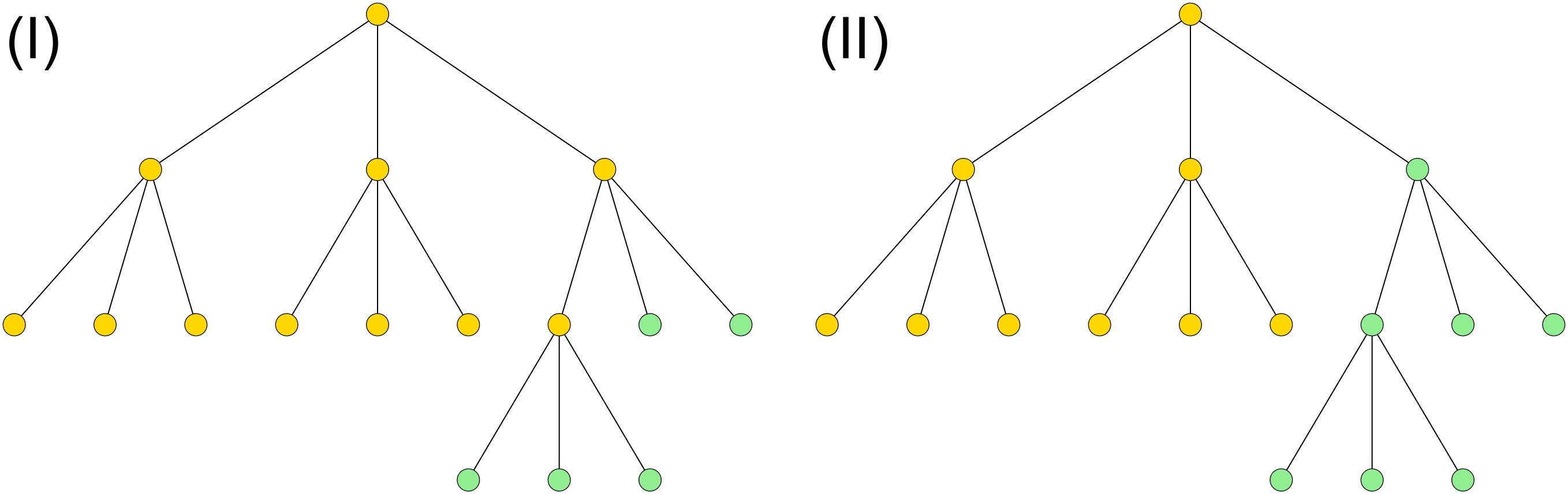
Scenario 1: Only one node at Level 2 has children belonging to Subtree 1

After Stage II, Subtree 1 (green) occupies the right-hand part of the tree and propagation reaches Level 1:

On Level 2, the two leaves L2C2 and L2C3 (children of L1C) belong to Subtree 1 from Stage I.
On Level 2, L2C1 (child of L1C) is a non-leaf that is promoted to Subtree 1 by Stage II (all of its Level-3 children belong to Subtree 1).
Since all children of L1C are now in Subtree 1, L1C is promoted to Subtree 1 as well.

All other nodes remain in Subtree 0 (gold).

In this scenario, continuing propagation by one more level is the expected outcome: introducing Subtree 1 at Level 1 via L1C preserves the same final leaf mapping while reducing split bookkeeping.

Extracted Split Parameters (Stage I only / before Stage II propagation):: {6; 0→1; 2} // API level 2 (L2*): two childless leaves under L1C are introduced (L2C2, L2C3)

{8; 0→1; 3} // API level 3 (L3*): the three leaves under L2C1 are introduced because L2C1 is still Subtree 0

Total: 2 operations and 5 cell updates.

Extracted Split Parameters (after Stage II):: {4; 0→1; 1} // API level 1 (L1*): introduce Subtree 1 via L1C (child of Root)

Total: 1 operation and 1 cell update.

Incorrect Stage II application (illustrative):

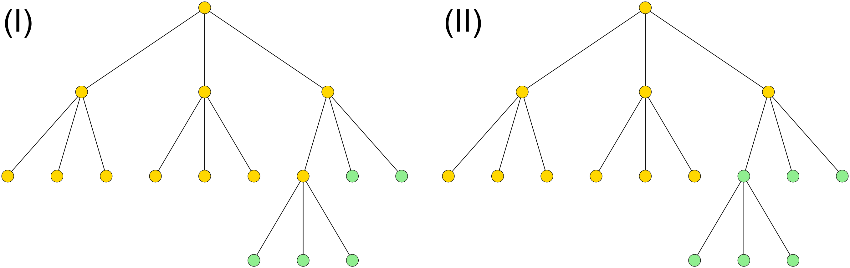
If propagation is stopped one level too early in Stage II, L1C is not promoted even though all its children are already in Subtree 1. The result is a Level-2 split that introduces L2C1, L2C2, and L2C3 instead of a single Level-1 introduction via L1C. The leaf-to-subtree mapping is unchanged, but bookkeeping is worse (3 introduced cells instead of 1), so this illustrates an incorrect Stage II application.

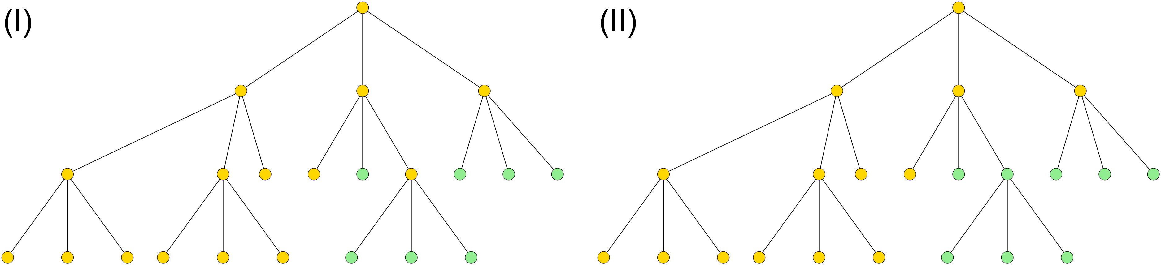
Scenario 2: Multiple nodes at Level 2 have children

After Stage II, Subtree 1 (green) remains represented on Level 2:

On Level 2, four leaves belong to Subtree 1 from Stage I (L2B2, L2C1, L2C2, L2C3).
On Level 2, L2B3 is a non-leaf that is promoted to Subtree 1 by Stage II (all of its Level-3 children belong to Subtree 1).

This yields one compact Level-2 introduction for Subtree 1 while keeping Level-1 parents in Subtree 0. In this scenario, this stopping point is expected and desirable: it realises the same final leaf mapping without creating an additional split on Level 1.

Extracted Split Parameters (Stage I only / before Stage II propagation):: {6; 0→1; 4} // API level 2 (L2*): 4 leaves introduced by Stage I (L2B2, L2C1, L2C2, L2C3)

{8; 0→1; 3} // API level 3 (L3*): 3 leaves introduced under L2B3 (parent still Subtree 0 before Stage II)

Total: 2 operations and 7 cell updates.

Extracted Split Parameters (after Stage II):: {6; 0→1; 5} // API level 2 (L2*): introduce Subtree 1 via L2B2, L2B3, L2C1, L2C2, L2C3

Total: 1 operation and 5 cell updates.

Incorrect Stage II application (illustrative):

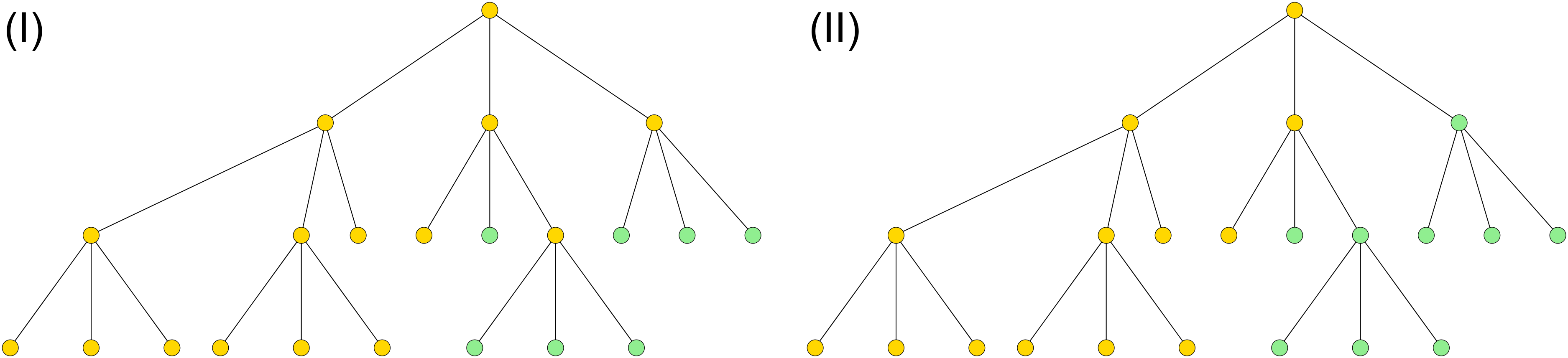
If propagation continues one level further than desired, L1C is promoted to Subtree 1 because all of its children are already green. However, L1B remains mixed, so the cells in Subtree 1 under L1B still require a Level-2 introduction. This creates two split levels (Level 1 and Level 2) instead of a single Level-2 split, i.e. more split operations for the same final leaf assignment.

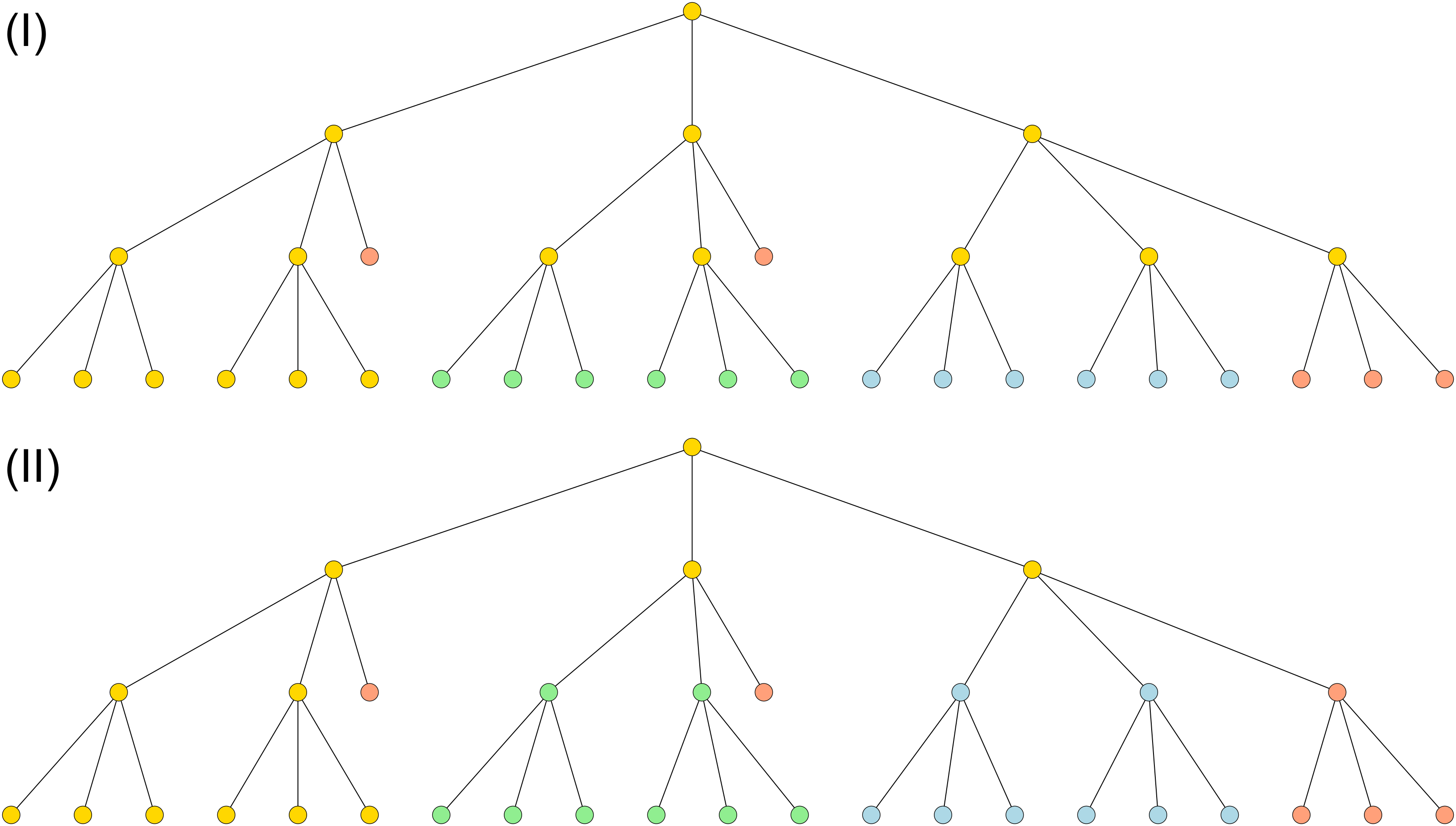
Scenario 3: A multi-way split across 4 subtrees after Stage II

For the fine-first BFS ordering, Stage I already yields contiguous Level-3 blocks for Subtrees 1 and 2, while Subtree 3 is composed of two childless Level-2 leaves and one refined Level-2 block. After Stage II, this structure is compacted on Level 2 by promoting uniform refined parents:

Subtree 1: refined L2B1 and L2B2 (6 Level-3 leaves total)
Subtree 2: refined L2C1 and L2C2 (6 Level-3 leaves total)
Subtree 3: childless leaves L2A3 and L2B3, plus refined L2C3 (3 Level-3 leaves) → 5 leaves total
Subtree 0: remaining leaves under refined L2A1 and L2A2 → 6 leaves total

The bottom-up propagation ensures strict parent-child consistency: only internal nodes whose full descendant set belongs to one subtree are promoted. Consequently, L2B1, L2B2, L2C1, L2C2, and L2C3 are promoted on Level 2, while L1A, L1B, and L1C are still resolved in Stage III.

Extracted Split Parameters (Stage I only / before Stage II propagation):: {8; 0→1; 6} // API level 3 (L3*): introduce Subtree 1 via all 6 leaves under L2B1 and L2B2

{8; 0→2; 6} // API level 3 (L3*): introduce Subtree 2 via all 6 leaves under L2C1 and L2C2

{6; 0→3; 2} // API level 2 (L2*): introduce Subtree 3 via childless leaves L2A3 and L2B3

{8; 0→3; 3} // API level 3 (L3*): introduce Subtree 3 via all 3 leaves under L2C3

Total: 4 operations and 17 cell updates.

Extracted Split Parameters (after Stage II):: {6; 0→1; 2} // API level 2 (L2*): introduce Subtree 1 via L2B1 and L2B2 (both refined)

{6; 0→2; 2} // API level 2 (L2*): introduce Subtree 2 via L2C1 and L2C2 (both refined)

{6; 0→3; 3} // API level 2 (L2*): introduce Subtree 3 via L2A3, L2B3 (childless) and L2C3 (refined)

Total: 3 operations and 7 cell updates.

Stage III (optional): Hierarchical Optimisation

The _optimize_hierarchy() function minimises the total number of split operations whilst preserving load balance established by Stage II. It does so by promoting a parent to the dominant child subtree when promotion is beneficial.

Algorithm

Iterative bottom-up optimisation over internal levels. On each pass, for each existing parent, the algorithm inspects all existing children and computes subtree frequencies. A promotion is applied only if:

all children exist for that parent (3^d children in dimension d),
children are mixed across at least two subtrees,
a dominant child subtree exists,
the dominant subtree differs from the current parent subtree,
promotion does not move ownership backward to an earlier subtree id,
and the dominant subtree has strictly higher child count than the current parent subtree count.

The process repeats until a full pass makes no changes.

Characteristics

Multi-pass iterative optimisation (converges when no further promotions are applicable)
Maintains Stage-II topology consistency (expects _propagate_bottom_up() to run first)
Preserves node existence flags (weight)
Changes only subtree assignments to reduce lower-level split pressure

Illustrative Scenarios of Hierarchically-Optimised Multi‑level Tree Splitting

The following diagrams show the same tree structure before and after applying hierarchical optimisation. This algorithm transforms the split structure to reduce the number of split operations whilst maintaining identical load distribution.

Scenarios 1–2: Why Stage III does not apply here:

In both scenarios, the Stage II result does not contain a set of introduced subtrees on some level \(L\) that forms a complete coarse block under a single common parent \(p\) on level \(L-1\). Any such promotion would either (i) recolour additional cells (changing the leaf-to-subtree mapping established by Stage II) or (ii) require additional corrective splits, i.e. it would not reduce split introductions.

More precisely, Stage III (“hierarchy lifting”) is only applicable if we can replace \(M\) split introductions of children on level \(L\) by a single split introduction of their parent on level \(L-1\) while preserving the leaf mapping. This is the “one parent’s worth”/complete-block condition (sum of children equals \(3^{d\cdot L}\) for one parent).

In Scenario 1, Stage II already yields a single Level-1 introduction (L1C). There is no lower-level set of introductions left that can be lifted further while reducing split count.
In Scenario 2, promoting L1C alone does not eliminate the Level-2 introduction needed for Subtree-1 cells under L1B; it would add another split level instead of reducing introductions.

Consequently, Scenarios 1 and 2 do not admit a correctness-preserving hierarchy lift that reduces split introductions.

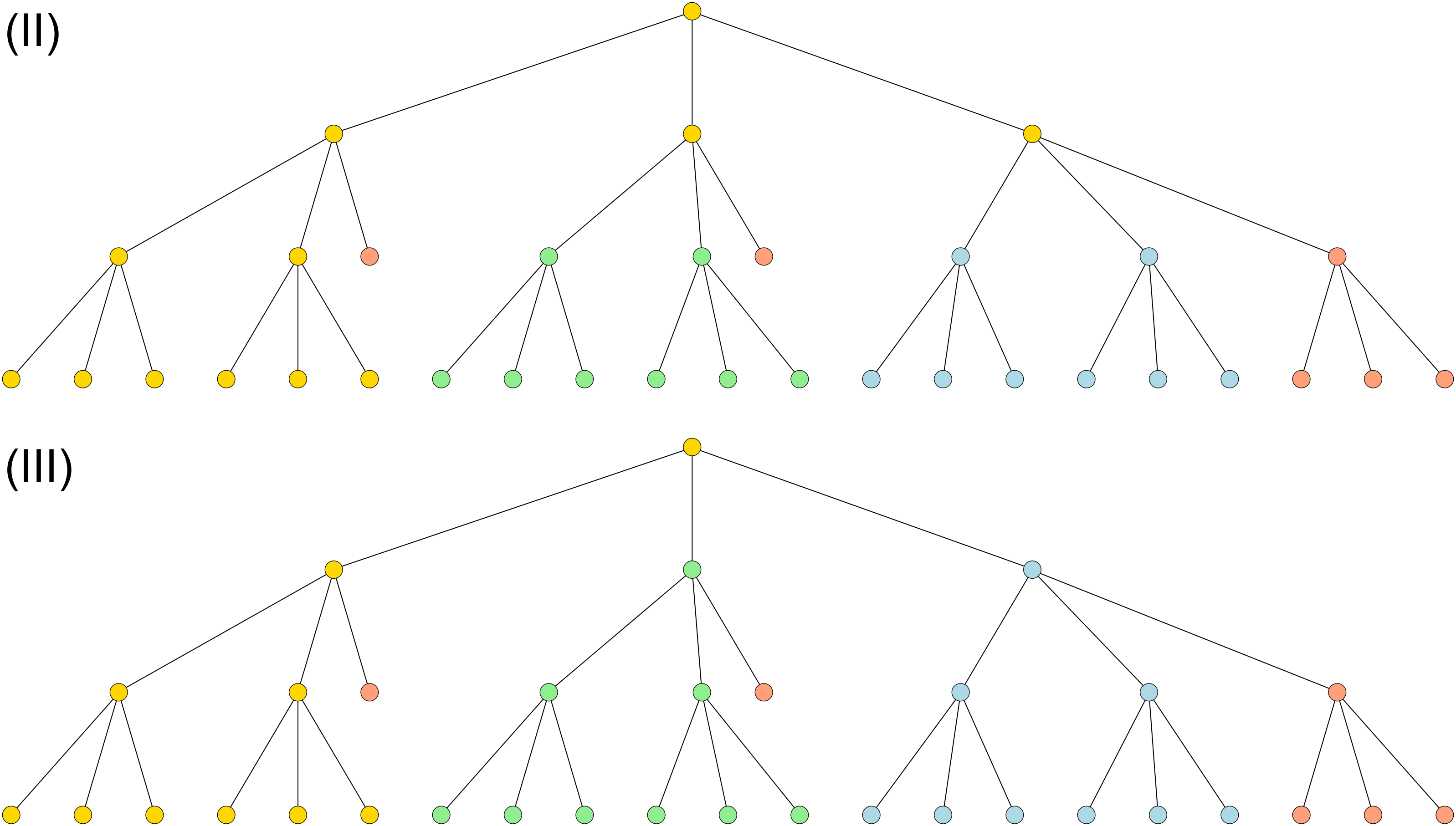
Scenario 3: A multi-way split across 4 subtrees after Stage III

In the fine-first BFS Scenario 3, Stage III lifts two compact Level-2 regions from Stage II to Level 1:

L1B is promoted to Subtree 1 (replacing the pair L2B1, L2B2)
L1C is promoted to Subtree 2 (replacing the pair L2C1, L2C2)
Subtree 3 remains represented on Level 2 through L2A3, L2B3, and L2C3

This preserves the Stage-II leaf mapping while reducing hierarchy depth for Subtrees 1 and 2.

Planned development

Stage III Implementation: Implement the (optional) third stage _optimize_hierarchy() in split_tree() as outlined above
Cost-Aware Splitting: Integration with splitting cost functions from Load balancing strategies
Hybrid Approaches: Configurable stage selection based on problem characteristics

Phase 3: Hardcoded parameter extraction (offline replay)

Stage IV translates the split tree into the constructor arguments of toolbox::loadbalancing::strategies::Hardcoded:

destination_ranks = Hardcoded.assign_trees_to_ranks_round_Robin(
    number_of_subtrees=tree.number_of_subtrees,
    max_ranks=number_of_ranks,
)
hardcoded_config, hardcoded_mode = Hardcoded.create_constructor_initialisation_string(
    tree,
    destination_ranks,
    modes=Hardcoded.BottomUp,   # optional: one marker, or one marker per split
)
project.set_load_balancing("toolbox::loadbalancing::strategies::Hardcoded", hardcoded_config)

Enumerated splits

The hardcoded strategy works with an enumerated list of splits. The _k_th split reads

‍Tree splitting_trees[k] hands number_of_cells[k] cells over to a new tree on rank destination_ranks[k], and it uses modes[k] to select these cells.

There is no notion of mesh sweeps. The C++ strategy hands out the splits in the order given and issues the _k_th split as soon as its splitting tree exists locally and holds more than number_of_cells[k] cells. See the class documentation of toolbox::loadbalancing::strategies::Hardcoded for all rules.

The lower-level helper extract_split_instructions() remains available for analysis/debugging and returns the raw lists (splitting_trees, number_of_cells, subtrees, bottom_up_flags):

splitting_trees: unique parent subtree id for all introduced cells of the split, or 0 if ambiguous.
number_of_cells: number of cells introduced by the split, i.e. cells with the target subtree id whose parent exists (level>0) and has a different subtree id. For level 0, it is the number of cells on level 0 that already belong to the target subtree.
subtrees: subtree ids introduced by the splits (not ranks).
bottom_up_flags: whether the split is a bottom-up split, i.e. whether the subtree is introduced on several levels.

The splits are ordered from coarse to fine levels and, within a level, by subtree id.

Split modes

Each split is either a top-down split (peano4::SplitInstruction::Mode::AggressiveTopDown) or a bottom-up split (peano4::SplitInstruction::Mode::BottomUp). Top-down splits hand over whole refined cells including their children as long as cells are still owed, i.e. the new tree might get a few cells more than requested. Bottom-up splits hand over fine grid cells one by one along the space-filling curve and hence reproduce the offline plan cell by cell. By default, create_constructor_initialisation_string() infers the modes from bottom_up_flags. The argument modes overwrites them with a single marker Hardcoded.TopDown or Hardcoded.BottomUp, or with one marker per split.

Ranks: one configuration, round-robin tree numbers

The constructor string is the same on all ranks. Each rank only keeps the splits whose splitting tree it hosts and drops all others, so splits of trees on other ranks never block a rank.

To tell which rank hosts a tree, the strategy relies on Peano's tree numbering, which is round robin: peano4::parallel::Node::getId() gives the n_th tree on rank _r the number n_·_R+_r_ for R ranks, and peano4::parallel::Node::getRank() maps tree number t onto rank t mod R. The offline decomposition refers to trees through their subtree numbers. We therefore always assume that subtree s lives on rank s mod R, i.e. that the subtrees are assigned to the ranks round robin, as assign_trees_to_ranks_round_Robin() does. Only then does a split of subtree s in the offline plan split tree s in Peano. create_constructor_initialisation_string() checks this and raises an error for any other assignment. It takes the number of ranks from the largest destination rank, unless you pass number_of_ranks.

Equivalent constructor usage in C++:

toolbox::loadbalancing::strategies::Hardcoded(
  {0, 0, 0},          // splitting_trees
  {182, 182, 182},    // number_of_cells
  {1, 2, 0},          // destination_ranks, round robin over three ranks
  peano4::SplitInstruction::Mode::BottomUp
);

Phase 4: Output and Visualisation

YAML Generation

The generate_tree_yaml function in src/toolbox/loadbalancing/api/strategies/SplitTrees.py creates comprehensive YAML files for Peano integration, containing:

Tree Structure: Complete spatial layout with (weight, subtree_id) tuples
Tree Metadata: Dimensions, refinement levels, domain boundaries, and leaf counts
Split Analysis: Subtree distribution statistics and load balancing results
Integration Data: All information required for Peano's hardcoded load balancer

These YAML files serve as the output format for integrating optimised decompositions back into Peano simulations.

For detailed YAML format specifications and generation parameters, see the generate_tree_yaml function documentation in src/toolbox/loadbalancing/api/strategies/SplitTrees.py.

Tree Visualisation

The API integrates with visualisation tools to generate graphical representations of tree structures in multiple formats:

Static Formats: High-resolution PDF and PNG files for publications and reports
Interactive Format: HTML files with zoom, pan, and hover capabilities using Plotly
Multi-level Display: Separate subplots showing each refinement level
Subtree Distinction: Colour-coded visualisation of different subtree assignments

The visualisation system automatically:

Adapts to Dimensions: Supports both 2D scatter plots and 3D visualisations
Scales Marker Sizes: Adjusts visual elements based on refinement level
Provides Hover Information: Shows detailed node information in interactive mode
Generates Responsive Layout: Creates full-width browser displays for analysis

For detailed implementation, customisation options, and technical specifications, see the TreeVisualizer module documentation in src/toolbox/loadbalancing/api/visualize/TreeVisualizer.py.

Main Script: OfflineDecomposition.py

The OfflineDecomposition.py script serves as the main interface for offline decomposition operations, providing command-line access to all API functionality.

Key Usage Patterns

# Analyse existing simulation data
python3 OfflineDecomposition.py -f /path/to/grid/files -d 3 -p
 
# Generate test cases for algorithm development
python3 OfflineDecomposition.py -d 2 -l 4 -p
 
# Apply load balancing optimisation
python3 OfflineDecomposition.py -d 3 -l 3 -s 4 -p
 
# Disable any Stage II and III update for leaf-only distribution
python3 OfflineDecomposition.py -d 3 -l 3 -s 4 --no-topology-update

Workflow Integration

The script integrates all API components into a complete workflow:

Phase 1: Input Generators via GridPatchFileReader or RegularGridGenerator, represented through the Tree data structure.
Phase 2: Splitting Strategies through SplitTrees, including Stage I (leaf distribution), Stage II (bottom-up propagation), and optional Stage III (hierarchical optimisation).
Phase 3: Hardcoded parameter extraction (offline replay) via Stage IV, i.e. create_constructor_initialisation_string(), to obtain (hardcoded_config, hardcoded_mode) for toolbox::loadbalancing::strategies::Hardcoded.
Phase 4: Output and Visualisation by exporting YAML (e.g. via generate_tree_yaml) plus optional visual artefacts for inspection and integration.

For complete command-line options, parameter details, and usage examples, see the OfflineDecomposition.py script documentation.

Output Files

The script generates several output files for analysis and integration:

Original YAML: Complete structure of the input tree before optimisation
Split YAML: Optimised tree structure after applying splitting strategies
Visualisation Files: PDF and PNG plots of tree structures (when visualisation is enabled)
Performance Metrics: Timing information for each processing stage

Performance Considerations

The API tracks and reports performance metrics for:

Input Processing Time: Time to read/generate tree structures
Visualisation Time: Time to create graphical representations
Splitting Time: Time to apply splitting algorithms
Total Processing Time: End-to-end processing duration

This enables analysis of scaling behaviour and identification of computational bottlenecks in the offline optimisation process.

Table of Contents