Advanced Usage of ExaGRyPE

Table of Contents

• Adding New Physics Scenarios
• Postprocessing On-the-fly
• Particles as Probes and Tracers
• Coupling Multiple Numerical Schemes (Solvers)

This section is designed to describe more user-defined options for those who are already familiar with the basic usage of ExaGRyPE.

Users are recommended to read and understand the Python/C++ scripts of the code before continuing here.

Adding New Physics Scenarios

For vacuum spacetimes, different physics scenarios are represented by different initial conditions. The initial conditions of ExaGRyPE can be assigned via a direct function, e.g., as done for the gauge wave scenario in src/exagrype/initialvalues/InitialValues.cpp. New analytical scenarios that are of general use belong into this file (and the namespace exagrype::initialvalues), so all ExaGRyPE applications can use them:

void exagrype::initialvalues::newScenario(
  double * __restrict__ Q, // Q[64+0],
  const tarch::la::Vector<Dimensions,double>&  x,
  double t
) {
  Q[0]  = 1.0;
  Q[1]  = ...... 
}

For more complicated initial conditions (e.g., black holes), users can introduce their own calculation library and include it before generating and building the Peano project. We also recommend defining a corresponding C++ flag to avoid potential linking issues when another scenario is picked. Such scenarios stay with your application rather than in the ExaGRyPE library. The TwoPunctures binding in src/exagrype/initialvalues/ApplyTwoPunctures.cpp is an example of such a calculator guarded by a flag.

peano4_project.output.makefile.add_cpp_file( "MyICCalculators/Calculator1.cpp" )
peano4_project.output.makefile.add_cpp_file( "MyICCalculators/Calculator2.cpp" )
......
peano4_project.output.makefile.add_CXX_flag( "-DIncludeMyCalculator" )
......

.......
#ifdef IncludeMyCalculator
#include "MyICCalculators/UseMyCalculator.h"
#endif
.......
void applications::exahype2::ccz4::newComplicatedScenario(
  double * __restrict__ Q, // Q[64+0],
  const tarch::la::Vector<Dimensions,double>&  x,
  double t
) {
  MyCalculator(Q, x, t);
}

Postprocessing On-the-fly

Users can define postprocessing functions if they wish to manipulate evolving variables during time stepping, or to extract more information from the system through material variables (material variables are additional variables that the user can ask the code to output alongside the evolving system into snapshots for inspection).

MySolver._auxiliary_variables = 3 #set the number of material variables you need
 
MySolver._my_user_includes += """
  #include "../MyPostprocessingfunctions.h"
"""
 
MySolver._preprocess_reconstructed_patch = """
  MyPostprocessingfunction(...);
  .......
"""
 
MySolver.create_data_structures()
MySolver.create_action_sets()

CCZ4.py and CCZ4Helper.py contain multiple postprocessing functions that users can use as examples to implement their own.

Particles as Probes and Tracers

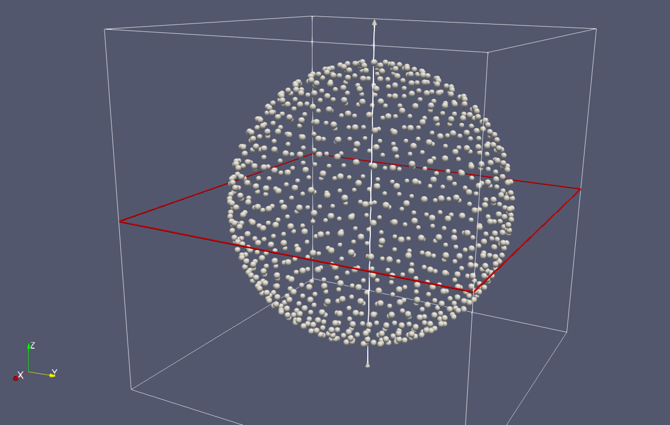
ExaGRyPE can have particles inserted into the domain for multiple purposes. These particles have no physics interaction and act as data probes or object tracers. To add particles to the domain, you can create a particle set using

tracer_particles = project.add_tracer( name="Tracer",attribute_count=59 )
init_action_set =  exahype2.tracer.InsertParticlesByCoordinates( 
    particle_set=tracer_particles, coordinates=[[0,0,8.0],[0,0,-8.0],[8.0,8.0,0],[-8.0,-8.0,0]])
init_action_set.descend_invocation_order = 0
project.add_action_set_to_initialisation( init_action_set )

besides specifying their coordinates directly, you can also import them from a file:

init_action_set = exahype2.tracer.InsertParticlesFromFile( 
    particle_set=tracer_particles, filename="t-design.dat", scale_factor=abs(offset[0])*0.8)

The next step is to associate the particles with your solver using the kernel you specify. For static data probes, the kernel only needs to specify how you project the neighbouring field solution onto your particle location; the most common one would be projectAllValuesOntoParticle_piecewiseLinear

tracer_action_set=exahype2.tracer.FiniteVolumesTracing(tracer_particles,
                                                       my_solver,
                                                       project_on_tracer_properties_kernel="::exahype2::fv::projectAllValuesOntoParticle_piecewiseLinear",
                                                       )
tracer_action_set.descend_invocation_order = my_solver._action_set_update_cell.descend_invocation_order+1
project.add_action_set_to_timestepping(tracer_action_set)
project.add_action_set_to_initialisation(tracer_action_set)

By switching to a projectAllValuesOntoParticle_piecewiseLinear_explicit_Euler kernel, you can ask particles to follow a certain vector field in the solution (or any variables as long as the total number equals the dimension number); this method can be used to trace objects flowing in the field, i.e., to track black holes moving in the merging binaries.

tracer_action_set=exahype2.tracer.FiniteVolumesTracing(tracer_particles,
                                                       my_solver,
                                                       project_on_tracer_properties_kernel="::exahype2::fv::projectAllValuesOntoParticle_piecewiseLinear_explicit_Euler",
                                                       projection_kernel_arguments="""marker,
                                                       {{PATCH_SIZE}},
                                                       {{NUMBER_OF_UNKNOWNS}}+{{NUMBER_OF_AUXILIARY_VARIABLES}},
                                                       fineGridCell{{SOLVER_NAME}}Q.value,
                                                       fineGridCell{{SOLVER_NAME}}CellLabel.getTimeStepSize(),
                                                       {17,18,19},
                                                       {-1,-1,-1},
                                                       *p
                                                       """)

The output of particles contains two parts: the first part is the usual vtu files showing the locations of particles and variables recorded by them; the second part is the csv file that you can control with

dump_action_set=exahype2.tracer.DumpTracerIntoDatabase(
    particle_set=tracer_particles,
    solver=my_solver,
    filename=args.path+"Tracer-BHTracker",
    number_of_entries_between_two_db_flushes=1000,
    output_precision=8,
    data_delta_between_two_snapsots=1e16,
    position_delta_between_two_snapsots=1e16,
    time_delta_between_two_snapsots=0.02,
    clear_database_after_flush      = True
    )
dump_action_set.descend_invocation_order = my_solver._action_set_compute_final_linear_combination.descend_invocation_order+2
project.add_action_set_to_timestepping(dump_action_set)

Each particle outputs its label, coordinates, time, and recorded data as a one-line entry each time the dumping criteria are satisfied; available criteria include entry count, data changes, position changes, and time changes. If the recorded entries exceed the threshold you specified (1000 in the example above), the code will output a csv file for the current data and clear the database.

We recommend outputting csv files every now and then during the simulation, as it helps reduce the memory footprint and is also safer, since a crash does not trigger automatic dumping, i.e., all particle data still in memory will be lost in that case.

Coupling Multiple Numerical Schemes (Solvers)

TODO