This tutorial studies a scenario where a regular mesh is a poor fit: a point explosion. A small region of high pressure in the middle of the domain releases a shock wave which travels outwards as a thin ring. Most of the domain remains at rest for most of the time, while the interesting physics happens within a few volumes around the front. Such setups call for adaptive mesh refinement (AMR), i.e. for a mesh which is fine where the solution is steep and coarse everywhere else.
We first set up a baseline on a regular mesh. It gives us a reference solution and shows where the regular mesh spends its effort. We run through the following steps:
- how to set up the point explosion with the same Euler solver as in A first advection problem with the Euler equations;
- how to run and visualise the explosion;
- how the solution evolves, and why the first-order scheme smears out the shock;
- how many patches actually hold steep gradients, i.e. how much work a regular mesh wastes.
We assume that you have completed A first advection problem with the Euler equations, as we reuse its flux and eigenvalue and skip most of the explanations of the script's structure.
The test case: a point explosion
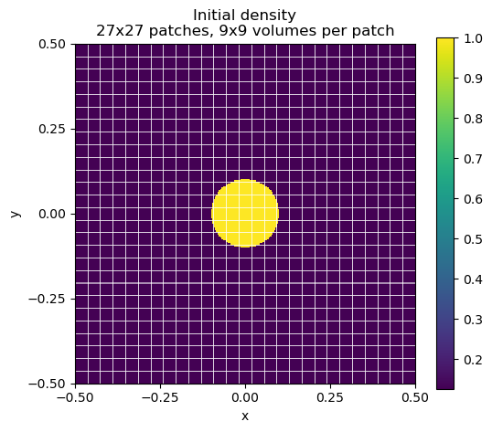
We solve the compressible Euler equations in two dimensions over the square \( [-0.5,0.5]^2\) . The gas is at rest everywhere. Within a circle of radius \( 0.1\) around the origin, density and pressure are high. Outside, they are low:
\begin{eqnarray*}
(\rho, u_1, u_2, p)(x,y,0) =
\begin{cases}
(1, 0, 0, 1) & \text{if } \sqrt{x^2+y^2} < 0.1, \\
(0.125, 0, 0, 0.1) & \text{otherwise.}
\end{cases}
\end{eqnarray*}
The states inside and outside are those of Sod's shock tube. Toro uses the same states for his cylindrical explosion test, with a radius of \( 0.4\) on the square \( [-1,1]^2\) (E. F. Toro: Riemann Solvers and Numerical Methods for Fluid Dynamics, Springer). We shrink the radius, so the explosion starts from an almost point-like region.
Once the simulation starts, three waves emerge from the edge of the circle:
- a shock which runs outwards and compresses the gas at rest;
- a contact discontinuity which follows the shock more slowly. It separates the gas from inside the circle from the gas that was outside;
- a rarefaction wave which runs inwards, reaches the centre and is reflected there. It leaves a region of low density behind.
There is no exact solution in closed form, but the setup is radially symmetric. The solution has to stay radially symmetric, too, which is a first sanity check of any simulation. With \( \gamma=1.4\) , the total energy is \( E = p/(\gamma-1)\) , as the gas is at rest initially.
Configuring the environment
As in the previous tutorials, we add the Python API to the search path:
import sys, os
sys.path.insert(0, os.path.abspath("../../src"))
import exahype2
try:
import ipywidgets, matplotlib
except ImportError:
!{sys.executable} -m pip install ipywidgets matplotlib
Project and solver
The project and the solver are the same as in A first advection problem with the Euler equations. Only the output directory changes. We need a flux, the maximum eigenvalue and a point-wise initial condition.
namespace = ["tutorials", "exahype2", "euler"],
project_name = "Euler",
directory = "13_euler-with-amr",
executable = "euler",
)
"EulerFV",
4,
0,
)
The conservative flux F(Q) of a hyperbolic PDE.
Point-wise initial condition: given the physical position of a single degree of freedom,...
The maximum absolute eigenvalue of the flux Jacobian in a given direction, i.e.
Abstract base class for all ExaHyPE 2 solvers.
Numerical scheme and mesh
We stick to Finite Volumes with a Rusanov flux and explicit Euler over patches of \( 9 \times 9\) volumes. The domain is five times wider than in A first advection problem with the Euler equations. With a maximum volume size of 0.005, ExaHyPE ends up with \( 27 \times 27\) patches, i.e. with \( 243 \times 243\) volumes, each of size \( 1/243 \approx 0.004\) .
patch_size = 9
volume_size = 0.005
solver,
first_plot_time_stamp = 0.0,
time_in_between_plots = 0.01,
)
Plotting counterpart to RusanovWithExplicitEuler: maps the patch data of a Finite Volume scheme with ...
Finite Volumes with a Rusanov Riemann solver and explicit Euler time stepping, realised over a block-...
Setup phase counterpart to RusanovWithExplicitEuler: sets the initial condition for a Finite Volume s...
The picture shows the initial density on this mesh. The white lines are the patch boundaries. The high-pressure region covers only a handful of patches:
Mesh and initial condition
Global simulation parameters
We simulate until \( t=0.2\) . By then, the shock has travelled to a radius of roughly \( 0.42\) , i.e. it has not reached the boundary yet. The boundary conditions therefore do not influence the solution, and we can pick the simplest option: a periodic domain. This way, we do not have to implement any boundary conditions.
project.add_solver(solver)
project.set_global_simulation_parameters(
dimensions = 2,
offset = [-0.5, -0.5],
size = [ 1.0, 1.0],
min_end_time = 0.2,
max_end_time = 0.2,
periodic_BC = [True, True, True],
)
Lowering into C++
project.set_Peano4_installation(os.path.abspath("../../"), peano4.api.output.CompileMode.RELEASE)
peano4_project = project.generate_Peano4_project(verbosity=peano4.api.LoggerVerbosity.TEXT)
peano4_project.generate()
Adding the actual physics
Flux and eigenvalue are exactly the same as in A first advection problem with the Euler equations, the physics does not change, only the scenario. The initial condition is new. It translates the primitive variables \( (\rho, u_1, u_2, p)\) from above into the conserved quantities \( Q = (\rho, \rho u_1, \rho u_2, E)\) .
Exercise:** Copy flux() and maxEigenvalue() from your solution of A first advection problem with the Euler equations into 13_euler-with-amr/EulerFV.cpp and implement initPointWisely(). If you want to skip the exercise, run the cell below. It overwrites the file with our reference implementation.
%%writefile 13_euler-with-amr/EulerFV.cpp
void tutorials::exahype2::euler::EulerFV::flux(
const double* __restrict__ Q, const tarch::la::Vector<Dimensions, double>& x, int normal, double* __restrict__ F
) {
const double irho = 1.0 / Q[0];
constexpr double gamma = 1.4;
const double p = (gamma - 1.0) * (Q[3] - 0.5 * irho * (Q[1] * Q[1] + Q[2] * Q[2]));
switch (normal) {
case 0:
F[0] = Q[1];
F[1] = irho * Q[1] * Q[1] + p;
F[2] = irho * Q[1] * Q[2];
F[3] = irho * Q[1] * (Q[3] + p);
break;
case 1:
F[0] = Q[2];
F[1] = irho * Q[2] * Q[1];
F[2] = irho * Q[2] * Q[2] + p;
F[3] = irho * Q[2] * (Q[3] + p);
break;
}
}
void tutorials::exahype2::euler::EulerFV::maxEigenvalue(
const double* __restrict__ Q, const tarch::la::Vector<Dimensions, double>& x, int normal, double* __restrict__ lambdaMax
) {
const double irho = 1.0 / Q[0];
constexpr double gamma = 1.4;
const double p = (gamma - 1.0) * (Q[3] - 0.5 * irho * (Q[1] * Q[1] + Q[2] * Q[2]));
const double c = std::sqrt(gamma * p * irho);
// velocity, i.e. momentum divided by density
const double u = Q[1 + normal] * irho;
lambdaMax[0] = std::max(std::abs(u + c), std::abs(u - c));
}
void tutorials::exahype2::euler::EulerFV::initPointWisely(
const tarch::la::Vector<Dimensions, double>& x, double* __restrict__ Q
) {
// Gas at rest. Sod's left state within a circle of radius 0.1 around
// the origin, Sod's right state outside.
constexpr double gamma = 1.4;
constexpr double radius = 0.1;
const bool inside = x[0] * x[0] + x[1] * x[1] < radius * radius;
const double rho = inside ? 1.0 : 0.125;
const double p = inside ? 1.0 : 0.1;
Q[0] = rho;
Q[1] = 0.0;
Q[2] = 0.0;
Q[3] = p / (gamma - 1.0);
}
Log filter, build and run
%%writefile 13_euler-with-amr/exahype2.log-filter
debug tarch -1 black always-on
debug peano4 -1 black always-on
debug exahype2 -1 black always-on
debug toolbox -1 black always-on
debug tutorials -1 black always-on
trace tarch -1 black always-on
trace peano4 -1 black always-on
trace exahype2 -1 black always-on
trace toolbox -1 black always-on
trace tutorials -1 black always-on
info tarch -1 white always-on
info peano4 -1 white always-on
info exahype2 -1 white always-on
info toolbox -1 white always-on
info tutorials -1 white always-on
!cd 13_euler-with-amr && make -j
!cd 13_euler-with-amr && ./euler
The run takes around half a minute and writes 21 snapshots into 13_euler-with-amr/solution-EulerFV.peano-patch-file plus the files it includes.
Interactive visualisation
We use the notebook viewer again. As the density drops quickly after the explosion, the colour range fixed by the first snapshot is not very helpful here. We therefore pick a narrower range by hand. Play around with the unknowns: The energy shows the shock very clearly, and the momenta show that the gas moves outwards.
"13_euler-with-amr/solution-EulerFV.peano-patch-file",
unknown = 0,
unknown_names = ["rho", "rho u_1", "rho u_2", "E"],
clim = (0.05, 0.4),
)
Interactive visualisation of Peano patch files within Jupyter notebooks.
show_solution(file_name, unknown=0, unknown_names=None, clim=None)
Interactive viewer for a patch file within a Jupyter notebook.
What we see
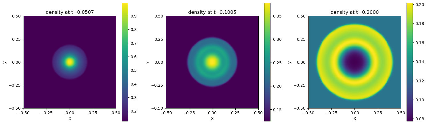
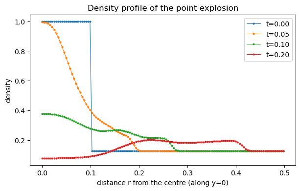
The pictures below show the density at three time stamps. Each one uses its own colour range. The solution stays radially symmetric. At \( t=0.05\) , the high density region in the centre has started to expand. At \( t=0.1\) , we see a ring of compressed gas behind the shock. At \( t=0.2\) , the rarefaction has emptied the centre, and the compressed gas forms a wide ring between a radius of roughly \( 0.2\) and the shock at roughly \( 0.42\) .
Density snapshots
The radial profile makes this more explicit. We plot the density along the positive \( x\) -axis. The initial jump at \( r=0.1\) breaks up into the waves described above. The shock at the right end of each profile is not a sharp jump, though: it is smeared over several volumes. This is the numerical diffusion of the first-order Rusanov scheme that we have already seen in A first advection problem with the Euler equations.
Radial density profile
Where the regular mesh wastes effort
To get a sharper shock, we have to make the volumes smaller. With a regular mesh, this is expensive: If we make the volumes three times smaller, we get nine times as many volumes in 2d. The time step size shrinks by a factor of three, too, due to the CFL condition. One refinement step therefore makes the simulation 27 times more expensive in 2d, and 81 times more expensive in 3d.
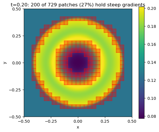
Yet, most of the mesh does not need this resolution. The picture below marks all patches in which the density jumps steeply between neighbouring volumes at the final time. Only around a quarter of the patches hold such steep gradients. Furthermore, this set of patches changes over time: early on, only a few patches in the centre are relevant. The region of interest then grows as a ring with the shock.
Patches with steep gradients
This is the motivation for adaptive mesh refinement: We want a mesh which is fine around the waves and coarse elsewhere, and which follows the waves as they travel through the domain. The regular-mesh solution of this tutorial serves as reference for such adaptive runs.
Exercise:** Reduce the volume size to 0.002 and rerun the notebook from the cell where we set up the mesh. ExaHyPE now uses \( 81 \times 81\) patches. Compare the runtime and the sharpness of the shock with the coarse run.
The pictures of this tutorial are created by the script tutorials/exahype2/illustrations/13_euler-with-amr.py, which runs exactly this experiment.
Point-wise adaptive mesh refinement for the initial condition
The initial condition is discontinuous only along the circle of radius 0.1. A first step towards AMR is therefore to refine the mesh around this circle while we set up the simulation, i.e. to make the mesh fine where the initial condition is steep, and to keep it coarse everywhere else.
ExaHyPE asks the user where to refine through a further PDE term: exahype2.api.RefineErasePointwisely. Like all the other terms, it is evaluated point-wisely, i.e. once per volume. It is handed the solution \( Q\) in the volume, the volume's centre \( x\) and the time stamp \( t\) , and it writes its decision into the output argument refinementCommand:
- exahype2::RefinementCommand::Refine asks for a finer mesh around \( x\) ;
- exahype2::RefinementCommand::Erase says that the mesh around \( x\) may become coarser;
- exahype2::RefinementCommand::Keep, which ExaHyPE sets before it calls the term, leaves the mesh as it is.
Our criterion is simple: We refine wherever the density exceeds 0.8, i.e. within the high-pressure region, and keep the mesh otherwise. The criterion is so short that we inject it directly from Python as a C++ snippet. We write the code into a separate directory 13_euler-with-amr-initial-refinement, so we can compare the outcome with the regular mesh.
namespace = ["tutorials", "exahype2", "euler"],
project_name = "Euler",
directory = "13_euler-with-amr-initial-refinement",
executable = "euler",
)
"EulerFV",
4,
0,
)
solver.add_pde_term(
implementation="if (Q[0] > 0.8) *refinementCommand = ::exahype2::RefinementCommand::Refine;",
)
)
Point-wise refinement criterion: given the solution Q at a single degree of freedom,...
Numerical scheme and adaptive mesh
We switch to exahype2.api.fv.SetupSimulationWithUserCodedRefinementCriterion as the generator which sets up the simulation. It takes two volume sizes:
- volume_size is the same parameter as for the regular mesh. The setup first constructs a regular mesh with volumes of at most this size. We start from a coarse mesh with \( 9 \times 9\) patches, i.e. volumes of size \( 1/81 \approx 0.012\) . The mesh never becomes coarser than this one.
- min_volume_size bounds the refinement: The setup refines a cell only if its volumes are at least of this size, i.e. the resulting volumes are strictly smaller than min_volume_size. Without such a bound, our criterion would refine the high-pressure region forever. With 0.002, the setup refines twice, down to volumes of size \( 1/729 \approx 0.0014\) .
On a regular mesh, volumes of size \( 1/729\) would mean \( 81 \times 81\) patches, i.e. 6561 of them.
On an adaptive mesh, a fine patch can be adjacent to a coarse patch. The face between the two is a hanging face: Peano does not store it, but creates it whenever a mesh sweep enters the fine cell and destroys it again once the sweep leaves the cell. The numerical scheme has to bridge the two resolutions there:
- Before the time step reconstructs the halo of a fine patch, it interpolates the data of the coarse face onto the hanging face. The constructor argument interpolation selects the scheme: piecewise constant or linear.
- Once the fine patches have projected their new solution onto their faces, the scheme restricts the data of the hanging faces onto the coarse face, where the coarse patch picks them up in the next time step. The argument restriction selects averaging or injection.
Linear interpolation and averaging are the default. We pass them explicitly, so you know where to change them.
The numerical scheme evaluates the refinement criterion at the end of each time step, too (we come back to this in the section on dynamic mesh refinement below). It takes its own bounds on the volume size, which are independent of the setup's: min_volume_size and max_volume_size. Without them, the time stepping would refine the high-pressure region further and further. We pass the setup's values, so the mesh which the setup has built remains as it is.
patch_size = 9
volume_size = 0.02
min_volume_size = 0.002
solver,
patch_size,
interpolation = toolbox.blockstructured.api.InterpolateHangingFaces.Scheme.Linear,
restriction = toolbox.blockstructured.api.RestrictHangingFaces.Scheme.Averaging,
min_volume_size = min_volume_size,
max_volume_size = volume_size,
)
solver,
volume_size = volume_size,
min_volume_size = min_volume_size,
)
solver,
first_plot_time_stamp = 0.0,
time_in_between_plots = 0.01,
)
Setup over a regular mesh which is then refined adaptively by the user's adaptivity criterion.
Global simulation parameters
We simulate until \( t=0.2\) , as on the regular mesh.
project.add_solver(solver)
project.set_global_simulation_parameters(
dimensions = 2,
offset = [-0.5, -0.5],
size = [ 1.0, 1.0],
min_end_time = 0.2,
max_end_time = 0.2,
periodic_BC = [True, True, True],
)
project.set_Peano4_installation(os.path.abspath("../../"), peano4.api.output.CompileMode.RELEASE)
peano4_project = project.generate_Peano4_project(verbosity=peano4.api.LoggerVerbosity.TEXT)
peano4_project.generate()
The setup task graph
The text output above lists the setup's task graph. The picture below shows the same graph.
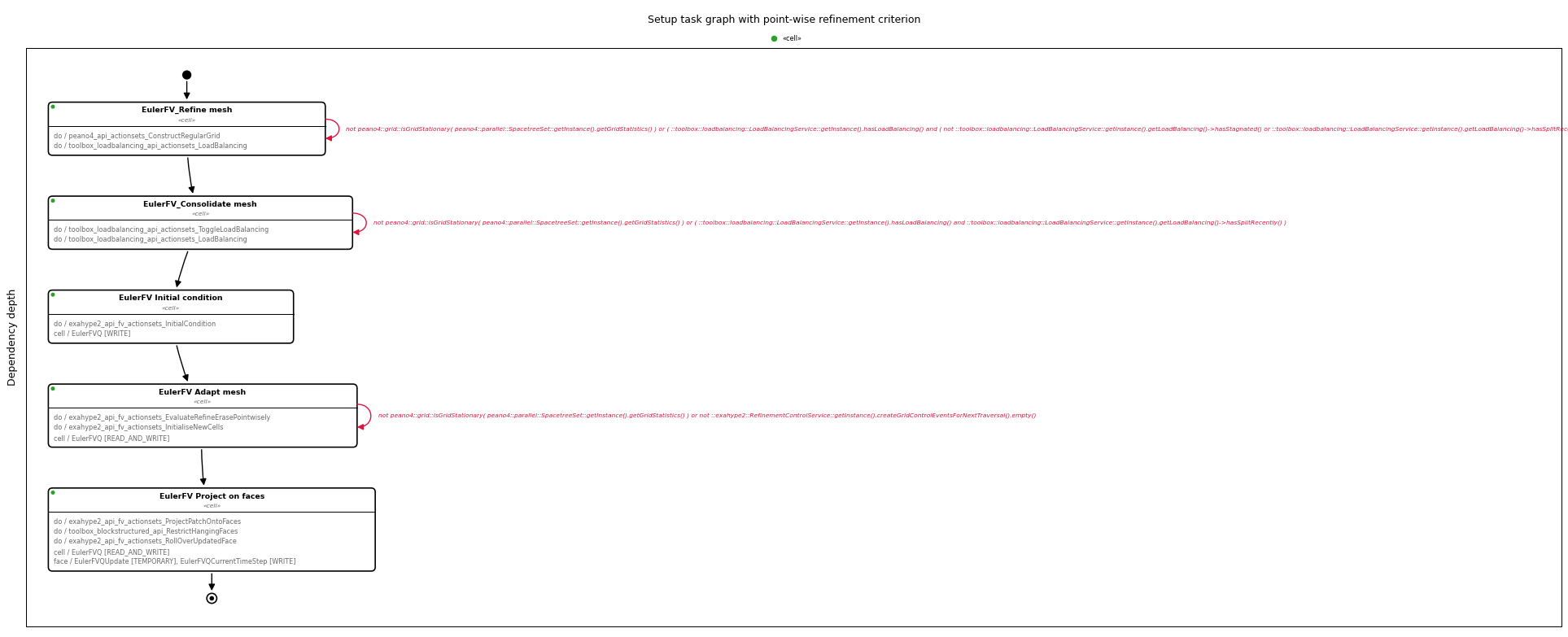
Setup task graph with point-wise refinement criterion
SetupSimulationWithUserCodedRefinementCriterion is a subclass of SetupSimulationOverRegularGrid, i.e. it first builds the same tasks as the setup over a regular mesh:
- Refine mesh constructs the regular mesh. The task repeats until the mesh is stationary (and the load balancing is happy).
- Consolidate mesh switches the load balancing off and waits until the last splits have been carried out.
- Initial condition invokes initPointWisely() in every volume.
The initial condition task carries the tag SetupSimulationOverRegularGrid.FinishedInitialRegularMeshSetup. After this task, the regular mesh holds the initial condition. The subclass searches for the tag and inserts its own task right after the tagged one. It uses the task graph's routine insert_after(), so the tasks which have followed the initial condition before now follow the new task:
- Adapt mesh is new. It repeats until the mesh is stationary, and it hosts two action sets. The first one evaluates refineErasePointwisely() in each volume of each cell. If any volume of a cell says Refine, it asks ExaHyPE's refinement service to refine this cell. If all volumes say Erase, it asks to erase the cell. The service collects these requests and hands them over to Peano. The second action set plugs into the creation of new cells and invokes initPointWisely() in each cell which the refinement adds to the mesh.
- Project on faces copies the solution from the cells onto the faces, as the first time step needs it there. It also restricts the data of the fine cells onto the coarse faces along the resolution transitions. It is the very last task of the setup, as it has to see the final mesh.
Peano does not refine a cell immediately. A refinement request issued in one mesh sweep makes Peano refine the mesh one to two sweeps later. Adapt mesh therefore repeats as long as the mesh changes or the refinement service still holds requests. Each refinement step evaluates the criterion again on the newly created cells, which in turn might ask for further refinement, until the cells are too small to be refined any further.
Adding the actual physics, build and run
The physics is the same as before, so we write the reference implementation of flux, eigenvalue and initial condition and the log filter into the new directory, build and run. As our refinement criterion has been injected from Python, EulerFV.cpp does not have to implement it.
%%writefile 13_euler-with-amr-initial-refinement/EulerFV.cpp
void tutorials::exahype2::euler::EulerFV::flux(
const double* __restrict__ Q, const tarch::la::Vector<Dimensions, double>& x, int normal, double* __restrict__ F
) {
const double irho = 1.0 / Q[0];
constexpr double gamma = 1.4;
const double p = (gamma - 1.0) * (Q[3] - 0.5 * irho * (Q[1] * Q[1] + Q[2] * Q[2]));
switch (normal) {
case 0:
F[0] = Q[1];
F[1] = irho * Q[1] * Q[1] + p;
F[2] = irho * Q[1] * Q[2];
F[3] = irho * Q[1] * (Q[3] + p);
break;
case 1:
F[0] = Q[2];
F[1] = irho * Q[2] * Q[1];
F[2] = irho * Q[2] * Q[2] + p;
F[3] = irho * Q[2] * (Q[3] + p);
break;
}
}
void tutorials::exahype2::euler::EulerFV::maxEigenvalue(
const double* __restrict__ Q, const tarch::la::Vector<Dimensions, double>& x, int normal, double* __restrict__ lambdaMax
) {
const double irho = 1.0 / Q[0];
constexpr double gamma = 1.4;
const double p = (gamma - 1.0) * (Q[3] - 0.5 * irho * (Q[1] * Q[1] + Q[2] * Q[2]));
const double c = std::sqrt(gamma * p * irho);
// velocity, i.e. momentum divided by density
const double u = Q[1 + normal] * irho;
lambdaMax[0] = std::max(std::abs(u + c), std::abs(u - c));
}
void tutorials::exahype2::euler::EulerFV::initPointWisely(
const tarch::la::Vector<Dimensions, double>& x, double* __restrict__ Q
) {
// Gas at rest. Sod's left state within a circle of radius 0.1 around
// the origin, Sod's right state outside.
constexpr double gamma = 1.4;
constexpr double radius = 0.1;
const bool inside = x[0] * x[0] + x[1] * x[1] < radius * radius;
const double rho = inside ? 1.0 : 0.125;
const double p = inside ? 1.0 : 0.1;
Q[0] = rho;
Q[1] = 0.0;
Q[2] = 0.0;
Q[3] = p / (gamma - 1.0);
}
%%writefile 13_euler-with-amr-initial-refinement/exahype2.log-filter
debug tarch -1 black always-on
debug peano4 -1 black always-on
debug exahype2 -1 black always-on
debug toolbox -1 black always-on
debug tutorials -1 black always-on
trace tarch -1 black always-on
trace peano4 -1 black always-on
trace exahype2 -1 black always-on
trace toolbox -1 black always-on
trace tutorials -1 black always-on
info tarch -1 white always-on
info peano4 -1 white always-on
info exahype2 -1 white always-on
info toolbox -1 white always-on
info tutorials -1 white always-on
!cd 13_euler-with-amr-initial-refinement && make -j
!cd 13_euler-with-amr-initial-refinement && ./euler
The adaptive mesh
The run takes a few minutes, as the finest volumes enforce small time steps: around 600 instead of 200 on the regular mesh. The first snapshot shows the initial condition on the adaptive mesh. The picture shows it together with the patch boundaries:
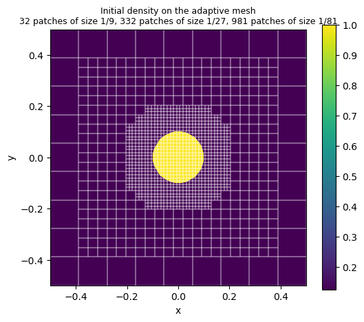
Initial density on the adaptive mesh
The volumes around the high-pressure region are as small as \( 1/729\) , while the volumes far away from it keep the size \( 1/81\) . The setup gets along with 1345 patches instead of 6561 for a regular mesh of the same finest resolution.
The refined region is wider than the circle where the density exceeds 0.8, though. Peano does not refine cells directly but vertices: if a vertex is refined, all cells adjacent to it are refined. A cell which asks for refinement thus also refines its neighbours. Each refinement level therefore adds a layer of fine cells around the region that the criterion has marked. This layer is welcome, as the explosion will spread out of the circle as soon as the simulation starts.
Time stepping on the adaptive mesh
The pictures below show the density at three time stamps together with the patch boundaries. The solution remains radially symmetric, even though it crosses two resolution transitions.
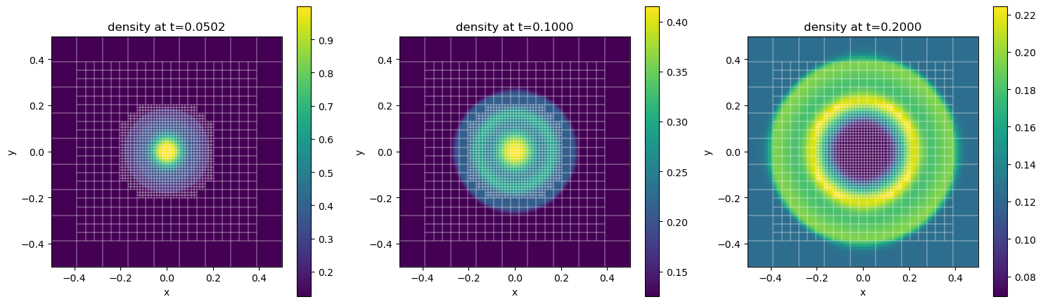
Density on the adaptive mesh
The mesh does not change over time: It is the mesh that the setup has constructed for the initial condition. The finest volumes cover the region around the initial explosion only. The comparison of the radial profiles with the regular mesh shows what this means:
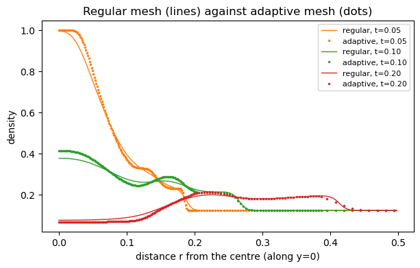
Regular against adaptive mesh
- At \( t=0.05\) and \( t=0.1\) , the waves still travel through the finest volumes. The adaptive run resolves the profile in the centre more sharply than the regular one, whose volumes are three times bigger. Where the waves cross from the finest to the next coarser volumes around \( r=0.2\) , the profile shows small kinks.
- At \( t=0.2\) , the shock sits at \( r \approx 0.42\) , i.e. it travels through volumes of size \( 1/243\) , which is the resolution of the regular mesh. The two runs hence yield almost the same shock.
The fluxes along a face between a coarse and a fine patch are not corrected, i.e. the scheme is not exactly conservative on adaptive meshes. The total mass in the domain changes by around \( 10^{-5}\) relative to its initial value until \( t=0.2\) .
To keep the shock within fine volumes all the time, the mesh has to follow the shock, i.e. we have to refine and erase while we run time steps.
You can inspect the outcome interactively, too:
"13_euler-with-amr-initial-refinement/solution-EulerFV.peano-patch-file",
unknown = 0,
unknown_names = ["rho", "rho u_1", "rho u_2", "E"],
clim = (0.05, 0.4),
)
Exercise:** Change the threshold of the refinement criterion or min_volume_size, rerun this part of the notebook, and study how the mesh changes. Switch to piecewise constant interpolation or to injection, and compare the profiles with the ones above.
Dynamic mesh refinement
So far, the mesh follows the initial condition only. ExaHyPE can also adapt the mesh while it runs time steps. The numerical schemes of exahype2.api.fv and exahype2.api.rkfd4 evaluate a RefineErasePointwisely term at the end of each time step, too. We have relied on this silently already: The time stepping above has evaluated our criterion after each time step, but all the cells with a density above 0.8 have been as fine as min_volume_size allows, so the criterion has never asked for any change.
To see the mesh change, we extend the criterion. Wherever the density drops below 0.1, the mesh may become coarser again:
- Initially, the density is 1 or 0.125, i.e. at least 0.125 everywhere. The criterion hence yields the same initial mesh as before.
- The rarefaction which runs inwards empties the centre of the domain. Once the density there drops below 0.1, the cells in the centre ask to be erased.
A cell asks to be erased only if all of its volumes say Erase. We write the code into a third directory, 13_euler-with-amr-dynamic.
namespace = ["tutorials", "exahype2", "euler"],
project_name = "Euler",
directory = "13_euler-with-amr-dynamic",
executable = "euler",
)
"EulerFV",
4,
0,
)
solver.add_pde_term(
implementation="""
if (Q[0] > 0.8) *refinementCommand = ::exahype2::RefinementCommand::Refine;
else if (Q[0] < 0.1) *refinementCommand = ::exahype2::RefinementCommand::Erase;
""",
)
)
Mesh size bounds and the mesh adaptation phase
The numerical scheme and the setup are the same as before. The scheme's volume size bounds now matter for both directions:
- min_volume_size: A cell asks for a refinement only if its volumes are at least of this size.
- max_volume_size: A cell asks to be erased only if the volumes of the coarser cell would be strictly smaller than this size. With the setup's volume_size, the mesh never becomes coarser than the initial regular mesh.
The scheme drops all other requests right away, so they never trigger any mesh adaptation. Without bounds, the mesh size is not constrained.
We also assign the solver's mesh adaptation explicitly. Without this line, the Finite Volume scheme would create the same one by default.
solver,
patch_size,
min_volume_size = min_volume_size,
max_volume_size = volume_size,
)
solver,
volume_size = volume_size,
min_volume_size = min_volume_size,
)
solver,
interpolation = toolbox.blockstructured.api.InterpolateAndRestrictCells.Interpolation.Linear,
restriction = toolbox.blockstructured.api.InterpolateAndRestrictCells.Restriction.Averaging,
)
solver,
first_plot_time_stamp = 0.0,
time_in_between_plots = 0.01,
)
Default mesh adaptation of the Finite Volume schemes.
Every ExaHyPE 2 project runs through four phases: the setup, the time stepping, the plotting and the mesh adaptation. The fourth one adapts the mesh and rebalances the load between two time steps:
- The very last task of each time step, Dynamic mesh refinement, evaluates refineErasePointwisely() in each volume and collects the refine and erase requests. It does not change the mesh itself. It also switches the load balancing on, which is switched off throughout the time step, and informs it that the time step has finished.
- Right after the time step, the main routine runs the mesh adaptation phase, but only if the time step has issued requests or if the load balancing has decided to split the mesh.
The solver's mesh adaptation, exahype2.api.fv.AdaptMeshAndBalanceLoad, contributes two tasks to this phase:
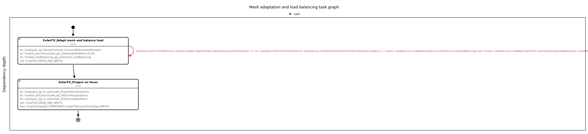
Mesh adaptation and load balancing task graph
- Adapt mesh and balance load repeats until the mesh is stationary, no requests are left and the load balancing does not split anymore. It hands the requests of the time step over to Peano without issuing new ones. If Peano creates a cell, the task interpolates the cell's patch from its parent (d-linearly by default). If Peano erases cells, the task averages their patches into their parent.
- Project on faces projects the patches onto the faces, as the new mesh has new faces.
If the mesh has changed, the time step size of the old mesh might violate the CFL condition on the new one. The mesh adaptation therefore sets the time step size to zero. The next time step does not advance in time, but it derives an admissible time step size from the new mesh, like the very first time step does.
We run until \( t=0.3\) this time, as the centre needs a while to become thin enough.
project.add_solver(solver)
project.set_global_simulation_parameters(
dimensions = 2,
offset = [-0.5, -0.5],
size = [ 1.0, 1.0],
min_end_time = 0.3,
max_end_time = 0.3,
periodic_BC = [True, True, True],
)
project.set_Peano4_installation(os.path.abspath("../../"), peano4.api.output.CompileMode.RELEASE)
peano4_project = project.generate_Peano4_project(verbosity=peano4.api.LoggerVerbosity.TEXT)
peano4_project.generate()
%%writefile 13_euler-with-amr-dynamic/EulerFV.cpp
void tutorials::exahype2::euler::EulerFV::flux(
const double* __restrict__ Q, const tarch::la::Vector<Dimensions, double>& x, int normal, double* __restrict__ F
) {
const double irho = 1.0 / Q[0];
constexpr double gamma = 1.4;
const double p = (gamma - 1.0) * (Q[3] - 0.5 * irho * (Q[1] * Q[1] + Q[2] * Q[2]));
switch (normal) {
case 0:
F[0] = Q[1];
F[1] = irho * Q[1] * Q[1] + p;
F[2] = irho * Q[1] * Q[2];
F[3] = irho * Q[1] * (Q[3] + p);
break;
case 1:
F[0] = Q[2];
F[1] = irho * Q[2] * Q[1];
F[2] = irho * Q[2] * Q[2] + p;
F[3] = irho * Q[2] * (Q[3] + p);
break;
}
}
void tutorials::exahype2::euler::EulerFV::maxEigenvalue(
const double* __restrict__ Q, const tarch::la::Vector<Dimensions, double>& x, int normal, double* __restrict__ lambdaMax
) {
const double irho = 1.0 / Q[0];
constexpr double gamma = 1.4;
const double p = (gamma - 1.0) * (Q[3] - 0.5 * irho * (Q[1] * Q[1] + Q[2] * Q[2]));
const double c = std::sqrt(gamma * p * irho);
// velocity, i.e. momentum divided by density
const double u = Q[1 + normal] * irho;
lambdaMax[0] = std::max(std::abs(u + c), std::abs(u - c));
}
void tutorials::exahype2::euler::EulerFV::initPointWisely(
const tarch::la::Vector<Dimensions, double>& x, double* __restrict__ Q
) {
// Gas at rest. Sod's left state within a circle of radius 0.1 around
// the origin, Sod's right state outside.
constexpr double gamma = 1.4;
constexpr double radius = 0.1;
const bool inside = x[0] * x[0] + x[1] * x[1] < radius * radius;
const double rho = inside ? 1.0 : 0.125;
const double p = inside ? 1.0 : 0.1;
Q[0] = rho;
Q[1] = 0.0;
Q[2] = 0.0;
Q[3] = p / (gamma - 1.0);
}
%%writefile 13_euler-with-amr-dynamic/exahype2.log-filter
debug tarch -1 black always-on
debug peano4 -1 black always-on
debug exahype2 -1 black always-on
debug toolbox -1 black always-on
debug tutorials -1 black always-on
trace tarch -1 black always-on
trace peano4 -1 black always-on
trace exahype2 -1 black always-on
trace toolbox -1 black always-on
trace tutorials -1 black always-on
info tarch -1 white always-on
info peano4 -1 white always-on
info exahype2 -1 white always-on
info toolbox -1 white always-on
info tutorials -1 white always-on
!cd 13_euler-with-amr-dynamic && make -j
!cd 13_euler-with-amr-dynamic && ./euler
The dynamically adaptive mesh
The number of patches over time shows when the mesh changes:
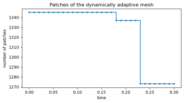
Patches of the dynamically adaptive mesh
The mesh changes twice: At \( t \approx 0.17\) , the centre has become thin enough, and ExaHyPE erases the finest patches of one cell in the very centre. At \( t \approx 0.23\) , it erases the finest patches of eight further cells, two along each axis on either side of the centre. The coarsened region hence forms a cross. The pictures show the density and the patch boundaries right before the first change and at the end of the simulation:
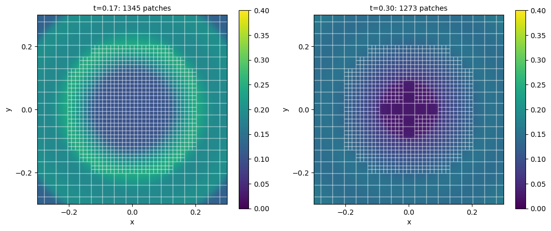
Mesh before the first coarsening and at the end
The coarsened region is much smaller than the region where the density is below 0.1, and it grows in steps of whole cells. Peano does not erase cells directly but vertices, and it is conservative: It erases the children of a cell only if all of them ask for it, and only if the same holds for all the cells of the same size around this cell. ExaHyPE mirrors this rule after each time step. It keeps an erase request only if Peano can realise it, and it drops all others right away. The mesh adaptation phase hence runs only twice until \( t=0.3\) , and it changes the mesh both times. As ExaHyPE hands Peano one request per cell which can be erased, the mesh remains rotationally symmetric, like the solution.
You can inspect the outcome interactively:
"13_euler-with-amr-dynamic/solution-EulerFV.peano-patch-file",
unknown = 0,
unknown_names = ["rho", "rho u_1", "rho u_2", "E"],
clim = (0.05, 0.4),
)
Exercise:** Enlarge the domain, run longer, and study how often the mesh changes. Switch the mesh adaptation to piecewise constant interpolation, and compare the solution after the coarsening. Finally, let the criterion refine around the shock, e.g. where the density exceeds 0.2, and observe how the mesh evolves.
The pictures of this section are created by the script tutorials/exahype2/illustrations/13_euler-with-amr.py, too.
Fourth-order Finite Differences need a smooth solution
So far, we have used the first-order Finite Volumes. The shock is smeared over several volumes, but the scheme remains stable. In Higher-order solvers: Runge Kutta and Finite Differences, we have met the fourth-order Finite Differences of exahype2.api.rkfd4, which converge way faster for smooth solutions. Different to the Finite Volumes, the central differences have no numerical diffusion. Across a discontinuity, they produce oscillations, and nothing damps them.
We can see this if we swap the numerical scheme of our point explosion for the Finite Differences, i.e. if we run the setup on the regular mesh with the rkfd4 classes from Higher-order solvers: Runge Kutta and Finite Differences. The oscillations around the initial jump grow within a few time steps until the pressure becomes negative or the maximum eigenvalue explodes. The CFL condition then shrinks the time step size by five orders of magnitude, and the simulation stalls at \( t \approx 0.006\) :
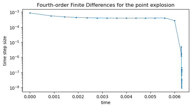
Time step sizes of the Finite Differences for the point explosion
For the Finite Differences, we therefore replace the explosion by a smooth Gaussian pulse. The gas is at rest, and density and pressure are raised around the origin:
\begin{eqnarray*}
\rho(x,y,0) = 1 + \frac{1}{2} e^{-r^2/w^2}, \qquad
u_1 = u_2 = 0, \qquad
p = \rho^\gamma,
\end{eqnarray*}
with \( r=\sqrt{x^2+y^2}\) and the width \( w=0.05\) . As the pressure follows the density isentropically, the pulse releases sound waves only. The pulse remains a high-pressure region in the centre, i.e. it behaves like a weak and smooth version of the explosion. On the regular mesh with grid cells of size \( 1/243\) , the width \( w\) spans twelve grid cells.
Project, solver and numerical scheme
The project gets a directory of its own, and the solver a new name, as it will no longer use Finite Volumes. The PDE terms are the same as for the Finite Volumes on the regular mesh:
namespace = ["tutorials", "exahype2", "euler"],
project_name = "Euler",
directory = "13_euler-with-amr-fd4",
executable = "euler",
)
"EulerFD4",
4,
0,
)
We pick the numerical scheme, the grid construction and the plotter from exahype2.api.rkfd4, exactly as in tutorials_exahype2_12_higher-order-solvers: fourth-order central differences with the classic fourth-order Runge-Kutta scheme over patches of \( 9 \times 9\) grid cells. With volume_size=0.005, the mesh is the same as the regular mesh of the Finite Volumes, i.e. \( 27 \times 27\) patches with \( 243 \times 243\) grid cells.
patch_size = 9
volume_size = 0.005
Fourth-order central Finite Differences with explicit Runge-Kutta time stepping, realised over a bloc...
Plotting counterpart of the fourth-order Finite Differences with Runge-Kutta time stepping (exahype2....
Setup phase of the fourth-order Finite Differences with Runge-Kutta time stepping (exahype2....
Global simulation parameters and code generation
We simulate until \( t=0.2\) again. By then, the sound waves have reached a radius of roughly \( 0.3\) , i.e. the periodic boundary does not influence the solution either.
project.add_solver(solver)
project.set_global_simulation_parameters(
dimensions = 2,
offset = [-0.5, -0.5],
size = [ 1.0, 1.0],
min_end_time = 0.2,
max_end_time = 0.2,
periodic_BC = [True, True, True],
)
project.set_Peano4_installation(os.path.abspath("../../"), peano4.api.output.CompileMode.RELEASE)
peano4_project = project.generate_Peano4_project(verbosity=peano4.api.LoggerVerbosity.TEXT)
peano4_project.generate()
Adding the actual physics, build and run
Flux and eigenvalue do not change, as the physics does not depend on the numerical scheme. Only the initial condition is new.
Exercise:** Implement initPointWisely() for the Gaussian pulse in 13_euler-with-amr-fd4/EulerFD4.cpp. If you want to skip the exercise, run the cell below. It writes our reference implementation into the file.
%%writefile 13_euler-with-amr-fd4/EulerFD4.cpp
void tutorials::exahype2::euler::EulerFD4::flux(
const double* __restrict__ Q, const tarch::la::Vector<Dimensions, double>& x, int normal, double* __restrict__ F
) {
const double irho = 1.0 / Q[0];
constexpr double gamma = 1.4;
const double p = (gamma - 1.0) * (Q[3] - 0.5 * irho * (Q[1] * Q[1] + Q[2] * Q[2]));
switch (normal) {
case 0:
F[0] = Q[1];
F[1] = irho * Q[1] * Q[1] + p;
F[2] = irho * Q[1] * Q[2];
F[3] = irho * Q[1] * (Q[3] + p);
break;
case 1:
F[0] = Q[2];
F[1] = irho * Q[2] * Q[1];
F[2] = irho * Q[2] * Q[2] + p;
F[3] = irho * Q[2] * (Q[3] + p);
break;
}
}
void tutorials::exahype2::euler::EulerFD4::maxEigenvalue(
const double* __restrict__ Q, const tarch::la::Vector<Dimensions, double>& x, int normal, double* __restrict__ lambdaMax
) {
const double irho = 1.0 / Q[0];
constexpr double gamma = 1.4;
const double p = (gamma - 1.0) * (Q[3] - 0.5 * irho * (Q[1] * Q[1] + Q[2] * Q[2]));
const double c = std::sqrt(gamma * p * irho);
// velocity, i.e. momentum divided by density
const double u = Q[1 + normal] * irho;
lambdaMax[0] = std::max(std::abs(u + c), std::abs(u - c));
}
void tutorials::exahype2::euler::EulerFD4::initPointWisely(
const tarch::la::Vector<Dimensions, double>& x, double* __restrict__ Q
) {
// Gas at rest. A Gaussian density pulse around the origin. The pressure
// follows the density isentropically, i.e. p = rho^gamma.
constexpr double gamma = 1.4;
constexpr double width = 0.05;
const double r2 = x[0] * x[0] + x[1] * x[1];
const double rho = 1.0 + 0.5 * std::exp(-r2 / (width * width));
const double p = std::pow(rho, gamma);
Q[0] = rho;
Q[1] = 0.0;
Q[2] = 0.0;
Q[3] = p / (gamma - 1.0);
}
%%writefile 13_euler-with-amr-fd4/exahype2.log-filter
debug tarch -1 black always-on
debug peano4 -1 black always-on
debug exahype2 -1 black always-on
debug toolbox -1 black always-on
debug tutorials -1 black always-on
trace tarch -1 black always-on
trace peano4 -1 black always-on
trace exahype2 -1 black always-on
trace toolbox -1 black always-on
trace tutorials -1 black always-on
info tarch -1 white always-on
info peano4 -1 white always-on
info exahype2 -1 white always-on
info toolbox -1 white always-on
info tutorials -1 white always-on
!cd 13_euler-with-amr-fd4 && make -j
!cd 13_euler-with-amr-fd4 && ./euler
The smooth pulse
The run takes a bit more than a minute and roughly 260 time steps, i.e. more than 1000 mesh sweeps, as each time step runs through the mesh once per Runge-Kutta stage. The pulse splits up: A ring of compressed gas travels outwards, and the density in the centre drops below its initial value behind the ring. The pictures show the density at three time stamps, each with its own colour range:
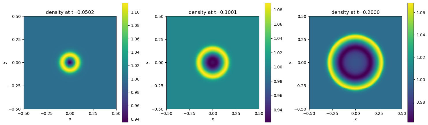
Density of the Gaussian pulse
The radial profile along the positive \( x\) -axis shows that the solution remains smooth. There are no oscillations, and the density stays between roughly \( 0.92\) and \( 1.11\) after the initial peak has dissolved. As the ring spreads over a larger and larger circle, its amplitude decays:
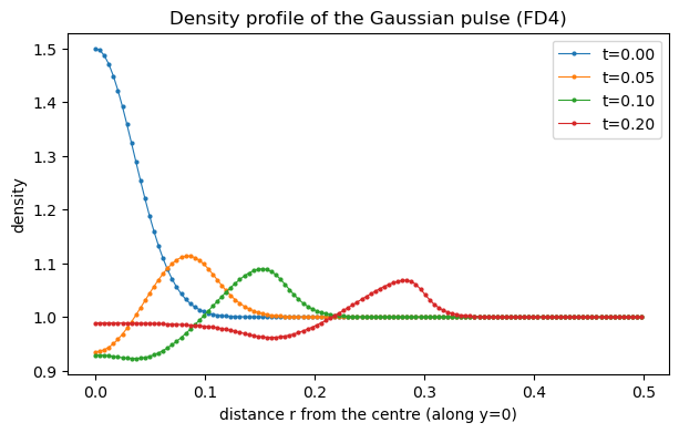
Radial density profile of the Gaussian pulse
You can inspect the outcome interactively:
"13_euler-with-amr-fd4/solution-EulerFD4.peano-patch-file",
unknown = 0,
unknown_names = ["rho", "rho u_1", "rho u_2", "E"],
)
Like the explosion, the pulse leaves most of the domain at rest. All the dynamics happen within a ring which is only a few times \( w\) wide. The Finite Differences would hence profit from an adaptive mesh as much as the Finite Volumes.
Exercise:** Switch the initial condition back to the point explosion, rerun the Finite Differences and observe how the time step size collapses. Then increase the amplitude of the Gaussian pulse step by step. The larger the amplitude, the faster the compression ring steepens into a shock, and the Finite Differences will break down again at some point.
The pictures of this section are created by the script tutorials/exahype2/illustrations/13_euler-with-amr.py. Pass –fd4-only to create only the pictures of this section.
Gradient-based mesh refinement
Our dynamic criterion refines where the density exceeds 0.8. This holds for the initial condition only: Once the shock runs outwards, its density is around 0.2, and the criterion does not see it anymore. The shock leaves the fine mesh, and the coarse mesh smears it out. We could lower the threshold, but the shock weakens as it expands: The density right behind it drops from 0.24 at \( t=0.05\) to 0.19 at \( t=0.25\) . At the same time, the gas further behind the shock reaches similar or even higher densities, e.g. 0.29 at \( t=0.1\) . A density threshold hence either loses the shock or refines most of the region behind it. What distinguishes the shock is its steep gradient.
ExaHyPE therefore offers a second adaptivity criterion, exahype2.api.GradientRefinement. Instead of refineErasePointwisely(), the solver then has a routine
void refineEraseWithGradient(
const double* __restrict__ gradient,
int normal,
);
which receives a difference quotient of all unknowns along the coordinate axis normal instead of the solution in one point:
- ExaHyPE calls the routine 2*Dimensions times per volume. For each axis, it passes the left difference quotient \( (Q_j - Q_{j-1})/h\) and the right one \( (Q_{j+1} - Q_j)/h\) , where \( h\) is the volume size.
- Volumes at the boundary of a patch have no neighbour on one side. For them, ExaHyPE passes the difference quotient towards the patch's interior in both calls.
- Each call starts from Keep. A volume asks for a refinement if any of its calls says Refine, and it may be erased only if all of its calls say Erase.
From there, everything works as before: A cell asks for a refinement if any of its volumes does, and to be erased if all of its volumes do. The volume size bounds and the mesh adaptation phase are the same as for the point-wise criterion.
We refine where the density changes by more than 5 per unit length, and we allow the mesh to become coarser where it changes by less than 1. The initial jump from 1 to 0.125 yields difference quotients of more than 40 even on the coarsest mesh, so the initial mesh is the same as before. We write the code into a fifth directory, 13_euler-with-amr-gradient:
namespace = ["tutorials", "exahype2", "euler"],
project_name = "Euler",
directory = "13_euler-with-amr-gradient",
executable = "euler",
)
"EulerFV",
4,
0,
)
solver.add_pde_term(
implementation="""
const double densityGradient = std::abs(gradient[0]);
if (densityGradient > 5.0) *refinementCommand = ::exahype2::RefinementCommand::Refine;
else if (densityGradient < 1.0) *refinementCommand = ::exahype2::RefinementCommand::Erase;
""",
)
)
Gradient-based refinement criterion: given a one-sided difference quotient of the solution along one ...
A solver may have at most one adaptivity criterion, i.e. either a RefineErasePointwisely or a GradientRefinement term. The setup and the numerical scheme pick the action set which evaluates the criterion from the criterion's type. For GradientRefinement, it is exahype2.api.blockstructured.DynamicMeshRefinementWithGradients. We hence do not have to change anything else: Numerical scheme, grid construction, mesh adaptation and plotter are the same as in the dynamic section. The Fourth-order Finite Differences have overwritten volume_size, so we set the mesh sizes again.
patch_size = 9
volume_size = 0.02
min_volume_size = 0.002
solver,
patch_size,
min_volume_size = min_volume_size,
max_volume_size = volume_size,
)
solver,
volume_size = volume_size,
min_volume_size = min_volume_size,
)
solver,
interpolation = toolbox.blockstructured.api.InterpolateAndRestrictCells.Interpolation.Linear,
restriction = toolbox.blockstructured.api.InterpolateAndRestrictCells.Restriction.Averaging,
)
solver,
first_plot_time_stamp = 0.0,
time_in_between_plots = 0.01,
)
project.add_solver(solver)
project.set_global_simulation_parameters(
dimensions = 2,
offset = [-0.5, -0.5],
size = [ 1.0, 1.0],
min_end_time = 0.3,
max_end_time = 0.3,
periodic_BC = [True, True, True],
)
project.set_Peano4_installation(os.path.abspath("../../"), peano4.api.output.CompileMode.RELEASE)
peano4_project = project.generate_Peano4_project(verbosity=peano4.api.LoggerVerbosity.TEXT)
peano4_project.generate()
The physics is the same as before. As the criterion is injected from Python, EulerFV.cpp does not contain it.
%%writefile 13_euler-with-amr-gradient/EulerFV.cpp
void tutorials::exahype2::euler::EulerFV::flux(
const double* __restrict__ Q, const tarch::la::Vector<Dimensions, double>& x, int normal, double* __restrict__ F
) {
const double irho = 1.0 / Q[0];
constexpr double gamma = 1.4;
const double p = (gamma - 1.0) * (Q[3] - 0.5 * irho * (Q[1] * Q[1] + Q[2] * Q[2]));
switch (normal) {
case 0:
F[0] = Q[1];
F[1] = irho * Q[1] * Q[1] + p;
F[2] = irho * Q[1] * Q[2];
F[3] = irho * Q[1] * (Q[3] + p);
break;
case 1:
F[0] = Q[2];
F[1] = irho * Q[2] * Q[1];
F[2] = irho * Q[2] * Q[2] + p;
F[3] = irho * Q[2] * (Q[3] + p);
break;
}
}
void tutorials::exahype2::euler::EulerFV::maxEigenvalue(
const double* __restrict__ Q, const tarch::la::Vector<Dimensions, double>& x, int normal, double* __restrict__ lambdaMax
) {
const double irho = 1.0 / Q[0];
constexpr double gamma = 1.4;
const double p = (gamma - 1.0) * (Q[3] - 0.5 * irho * (Q[1] * Q[1] + Q[2] * Q[2]));
const double c = std::sqrt(gamma * p * irho);
// velocity, i.e. momentum divided by density
const double u = Q[1 + normal] * irho;
lambdaMax[0] = std::max(std::abs(u + c), std::abs(u - c));
}
void tutorials::exahype2::euler::EulerFV::initPointWisely(
const tarch::la::Vector<Dimensions, double>& x, double* __restrict__ Q
) {
// Gas at rest. Sod's left state within a circle of radius 0.1 around
// the origin, Sod's right state outside.
constexpr double gamma = 1.4;
constexpr double radius = 0.1;
const bool inside = x[0] * x[0] + x[1] * x[1] < radius * radius;
const double rho = inside ? 1.0 : 0.125;
const double p = inside ? 1.0 : 0.1;
Q[0] = rho;
Q[1] = 0.0;
Q[2] = 0.0;
Q[3] = p / (gamma - 1.0);
}
%%writefile 13_euler-with-amr-gradient/exahype2.log-filter
debug tarch -1 black always-on
debug peano4 -1 black always-on
debug exahype2 -1 black always-on
debug toolbox -1 black always-on
debug tutorials -1 black always-on
trace tarch -1 black always-on
trace peano4 -1 black always-on
trace exahype2 -1 black always-on
trace toolbox -1 black always-on
trace tutorials -1 black always-on
info tarch -1 white always-on
info peano4 -1 white always-on
info exahype2 -1 white always-on
info toolbox -1 white always-on
info tutorials -1 white always-on
!cd 13_euler-with-amr-gradient && make -j
!cd 13_euler-with-amr-gradient && ./euler
Point-wise against gradient-based refinement
We compare the run against the dynamic run with the point-wise criterion. Both start from the same mesh, use the same volume size bounds and run until \( t=0.3\) . The density along the positive x-axis shows the difference:
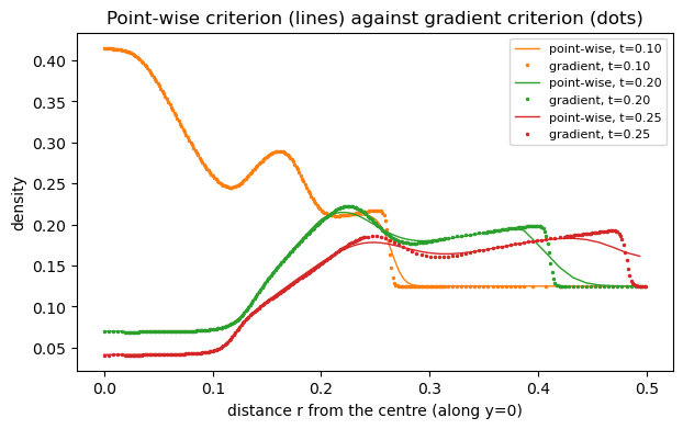
Density profiles of the point-wise and the gradient criterion
The two runs agree within the rarefaction, i.e. for \( r < 0.2\) . They differ at the shock. With the point-wise criterion, the shock runs on the coarse mesh from \( t \approx 0.1\) on. The scheme smears it over more and more volumes, and its peak decays faster. With the gradient criterion, the mesh follows the shock. It remains steep, and the density right behind it is higher: 0.193 instead of 0.182 at \( t=0.25\) . The smeared shock also lags behind slightly, i.e. its front is at \( r \approx 0.47\) instead of \( r \approx 0.48\) . At \( t=0.25\) , the shock is close to the boundary of the domain. As the domain is periodic, it collides with the shocks of the neighbouring explosions shortly after, so we compare until \( t=0.25\) only.
The pictures show the density and the patches in one quadrant of the domain at \( t=0.2\) :
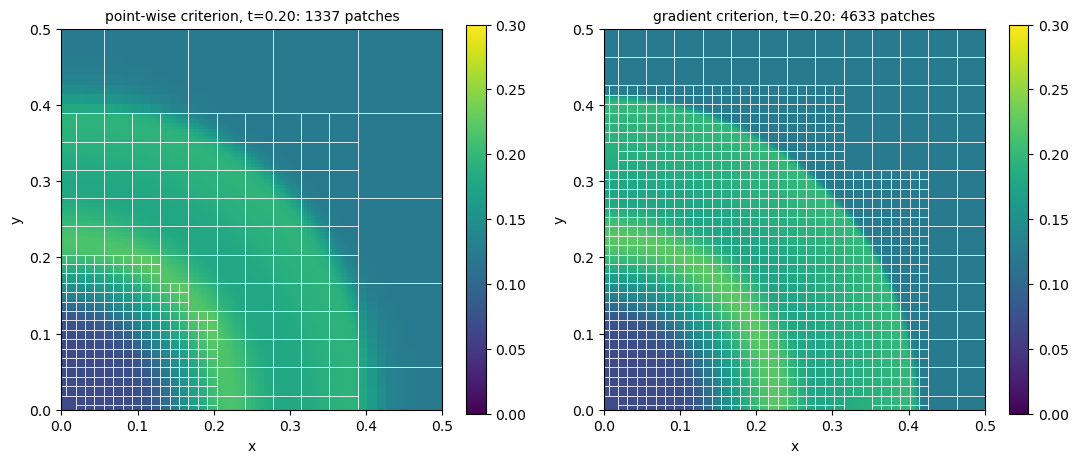
Meshes of the point-wise and the gradient criterion
The point-wise criterion has kept the fine mesh around the initial explosion. The shock has left it. The gradient criterion has refined the mesh around the shock. The fine region is not a thin ring around the shock though, but covers most of the region the shock has passed. This results from the two thresholds. Behind the shock, the density still changes by more than 1 per unit length in most places. The criterion there says neither Refine nor Erase, i.e. Keep. Furthermore, Peano erases a cell only if all of its siblings can be erased, too.
The accuracy comes at a price. The number of patches over time shows how much work each run does:
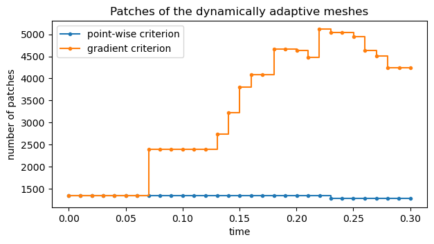
Number of patches of the point-wise and the gradient criterion
With the point-wise criterion, the mesh hardly changes. It erases a few cells in the centre later on, as we have seen before, and ends with 1273 patches. With the gradient criterion, the mesh hardly changes until \( t \approx 0.07\) , when the shock leaves the initially refined region and runs into the coarse mesh. From there, the mesh grows with the shock's circumference to more than 5000 patches at \( t \approx 0.22\) . Afterwards, the rarefaction behind the shock flattens, and the mesh becomes coarser there again. The run ends with 4249 patches, i.e. more than three times as many as the point-wise run. This is still less than the \( 81 \times 81 = 6561\) patches which a regular mesh with the finest patches would need. As for the other adaptive runs, the total mass changes by less than \( 10^{-5}\) relative to its initial value.
You can inspect the outcome interactively:
"13_euler-with-amr-gradient/solution-EulerFV.peano-patch-file",
unknown = 0,
unknown_names = ["rho", "rho u_1", "rho u_2", "E"],
clim = (0.05, 0.4),
)
Exercise:** Raise the erase threshold from 1 to 2 or 3, and study how the fine region and the number of patches change. Then let the criterion look at the pressure instead of the density, or at the gradient relative to the density, i.e. \( |\partial_i \rho| / \rho\) . Finally, let the point-wise criterion refine around the shock, e.g. where the density exceeds 0.2, and compare its mesh with the gradient criterion's.
The pictures of this section are created by the script tutorials/exahype2/illustrations/13_euler-with-amr.py, too. Pass –gradient-only to create only the pictures of this section.

 1.9.8