Symbolic names in the output
In A tsunami simulation with source code injection, SymPy, material parameters, non-conservative fluxes, and external files, we gave the unknowns of a solver symbolic names such as h, hu and hv. ExaHyPE writes these names into its output files, and Peano's postprocessing tools pick them up: the conversion into VTK labels the data with them, the point probe uses them as column names, and the notebook viewer offers them in its dropdown.
Preparing a data set
We rerun the "fake" tsunami over a flat sea floor from A tsunami simulation with source code injection, SymPy, material parameters, non-conservative fluxes, and external files, i.e. a solver with the unknowns h, hu and hv plus the auxiliary variable b:
import sys, os
sys.path.insert(0, os.path.abspath("../../src"))
import exahype2
namespace = ["tutorials", "exahype2", "postprocessing"],
project_name = "Tsunami",
directory = "41_postprocessing",
executable = "tsunami",
)
"SWE",
{"h": 1, "hu": 1, "hv": 1},
{"b": 1},
)
solver.add_user_solver_includes("#include <cmath>\n#include <algorithm>\n")
implementation = """
constexpr double g = 9.81;
const double h = Q[Variables::h];
const double un = Q[Variables::hu + normal] / h;
F[Variables::h] = Q[Variables::hu + normal];
F[Variables::hu] = Q[Variables::hu] * un;
F[Variables::hv] = Q[Variables::hv] * un;
F[Variables::hu + normal] += 0.5 * g * h * h;
""",
stateless = False,
))
implementation = """
constexpr double g = 9.81;
const double h = Q[Variables::h];
const double un = Q[Variables::hu + normal] / h;
lambdaMax[0] = std::abs(un) + std::sqrt(g * h);
""",
stateless = False,
))
implementation = """
Q[Variables::h] = 1.0 + 0.1 * std::exp(-100.0 * (x[0] * x[0] + x[1] * x[1]));
Q[Variables::hu] = 0.0;
Q[Variables::hv] = 0.0;
Q[Variables::b] = 0.0;
""",
stateless = False,
))
solver,
first_plot_time_stamp = 0.0,
time_in_between_plots = 0.05,
)
project.add_solver(solver)
project.set_global_simulation_parameters(
dimensions = 2,
offset = [-1.0, -1.0],
size = [ 2.0, 2.0],
min_end_time = 0.4,
max_end_time = 0.4,
periodic_BC = [True, True, True],
)
project.set_Peano4_installation(os.path.abspath("../../"), peano4.api.output.CompileMode.RELEASE)
peano4_project = project.generate_Peano4_project()
peano4_project.generate()
The conservative flux F(Q) of a hyperbolic PDE.
Point-wise initial condition: given the physical position of a single degree of freedom,...
The maximum absolute eigenvalue of the flux Jacobian in a given direction, i.e.
Abstract base class for all ExaHyPE 2 solvers.
Plotting counterpart to RusanovWithExplicitEuler: maps the patch data of a Finite Volume scheme with ...
Finite Volumes with a Rusanov Riemann solver and explicit Euler time stepping, realised over a block-...
Setup phase counterpart to RusanovWithExplicitEuler: sets the initial condition for a Finite Volume s...
!cd 41_postprocessing && make -j > make.log 2>&1 && ./tsunami > run.log 2>&1 && echo "done"
Names in the patch files
The plotter writes one patch file per snapshot. Its header describes the data:
!head -14 41_postprocessing/solution-SWE-0.peano-patch-file
The description holds the names of all entries of Q, i.e. of the unknowns followed by the auxiliary variables, as comma-separated list. A variable with multiplicity, such as a velocity {"v": 2}, shows up as v[0], v[1]. If a solver's variables have no names, the description holds the name of the data set instead, i.e. SWEQ.
The tools treat the description as list of names if and only if it holds one C++ identifier, optionally followed by an index such as [0], per unknown. Any other description is free text, which the tools ignore.
Converting into VTK
We convert the patch files into VTK files as usual. The conversion is documented in the offline conversion. It is chatty, so we only show its last line:
!cd 41_postprocessing && PYTHONPATH=../../../src {sys.executable} -m
tarch.plotter.api.render --split-unknowns solution-SWE.peano-patch-file | tail -1
Each snapshot yields one vtu file, and solution-SWE.SWEQ.pvd ties them together. Let's look into the arrays of one of them:
import vtk
def read_vtu(file_name):
reader = vtk.vtkXMLUnstructuredGridReader()
reader.SetFileName(file_name)
reader.Update()
return reader.GetOutput()
grid = read_vtu("41_postprocessing/solution-SWE.SWEQ-4.vtu")
cell_data = grid.GetCellData()
for i in range(cell_data.GetNumberOfArrays()):
array = cell_data.GetArray(i)
print(
f"{array.GetName():40} components:",
[array.GetComponentName(c) for c in range(array.GetNumberOfComponents())],
)
The array Unknowns holds all entries of Q plus the number of the subdomain, i.e. the rank, which wrote the data. Its components carry the names. In Paraview, open solution-SWE.SWEQ.pvd and colour by this array: the dropdown next to it then offers h, hu, hv, b and subdomain rather than 0, 1, 2, 3 and 4.
The option –split-unknowns additionally adds one array per variable. Paraview's filters such as Calculator, Contour or Threshold can then address h directly by its name. A variable with multiplicity becomes one vector array, i.e. v[0] and v[1] form the vector v. As Paraview only treats arrays with three components as vectors, e.g. to draw glyphs, the conversion pads two-dimensional vectors with a zero. The extra arrays roughly double the file size, which is why they are optional.
We can pick arrays by name in our own scripts, too. Here, we plot the momentum in x-direction:
import matplotlib.pyplot as plt
from vtk.util.numpy_support import vtk_to_numpy
def plot_array(grid, name, ax):
centres = vtk.vtkCellCenters()
centres.SetInputData(grid)
centres.Update()
xyz = vtk_to_numpy(centres.GetOutput().GetPoints().GetData())
values = vtk_to_numpy(grid.GetCellData().GetArray(name))
image = ax.tripcolor(xyz[:, 0], xyz[:, 1], values, shading="gouraud")
ax.set_aspect("equal")
ax.set_xlabel("x")
ax.set_ylabel("y")
ax.set_title(name)
ax.figure.colorbar(image, ax=ax)
fig, ax = plt.subplots(figsize=(6, 5))
plot_array(grid, "hu", ax)
plt.show()
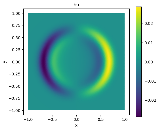
Momentum hu at t=0.2, picked by name from the converted VTK file
Right of the centre, the water flows in positive x-direction, left of the centre in negative x-direction.
The picture is created by tutorials/exahype2/illustrations/41_postprocessing.py, which runs exactly this setup.
Probing
The point probe extracts the values at one point over time into a CSV file (see its documentation). It uses the names as column headers:
!cd 41_postprocessing && PYTHONPATH=../../../src {sys.executable} -m
tarch.plotter.api.probe --point 0.5 0.0 -o probe.csv solution-SWE.peano-patch-file > /dev/null
with open("41_postprocessing/probe.csv") as csv_file:
print("".join(csv_file.readlines()[:4]))
If two data sets in the same files use the same name, the probe prefixes the names with the data set, e.g. SWEQ_h. Data without names yields SWEQ_0, SWEQ_1, and so forth.
The notebook viewer
The interactive viewer from tarch.plotter.api.notebook reads the names from the patch files, too, and offers them in its dropdown:
Interactive visualisation of Peano patch files within Jupyter notebooks.
show_solution(file_name, unknown=0, unknown_names=None, clim=None)
Interactive viewer for a patch file within a Jupyter notebook.

 1.9.8