 |
Peano
|
|
Peano
|
In A first advection problem with the Euler equations, we wrote the physics into a C++ file that ExaHyPE generated for us. This tutorial shows other ways to bring the physics in. We simulate the shallow water equations and
We start with a "fake" tsunami over a flat sea floor: a hump of water which collapses and sends a circular wave through a periodic basin. We then model the same setup with SymPy, and finally give the basin a sea floor with some structure, which we take from an external file. In the last step, the sea floor shapes how the tsunami spreads.
The shallow water equations describe a fluid whose horizontal length scales are much bigger than its depth, such as a tsunami crossing an ocean. We track the water height \( h\) and the momenta \( hu_1\) and \( hu_2\) :
\begin{eqnarray*} \frac{\partial}{\partial t} \begin{pmatrix} h \\ h u_1 \\ h u_2 \end{pmatrix} + \nabla \cdot \begin{pmatrix} h u_1 & h u_2 \\ h u_1^2 + \frac{1}{2} g h^2 & h u_1 u_2 \\ h u_2 u_1 & h u_2^2 + \frac{1}{2} g h^2 \end{pmatrix} + \begin{pmatrix} 0 \\ g h \, \partial_x b \\ g h \, \partial_y b \end{pmatrix} = \vec{0}, \end{eqnarray*}
with the gravity \( g=9.81\) and the bathymetry \( b\) , i.e. the height of the sea floor. The bathymetry does not change over time. It is therefore not an unknown but an auxiliary variable. In this first version, the sea floor is flat, i.e. \( b=0\) and the last term vanishes.
The eigenvalues of the flux in direction \( n\) are \( u_n - \sqrt{gh}\) , \( u_n\) and \( u_n + \sqrt{gh}\) . A wave on water at rest therefore travels with \( \sqrt{gh}\) , which is around 3.13 for \( h=1\) .
We start from water at rest with a small Gaussian hump in the centre of the domain \( [-1,1]^2\) :
\begin{eqnarray*} h(x,y,0) = 1 + 0.1 \exp\left( -100 (x^2+y^2) \right). \end{eqnarray*}
In A first advection problem with the Euler equations, we told ExaHyPE that there are four unknowns, and it was our job to remember that Q[1] is the momentum in x-direction. This time, we give each unknown and each auxiliary variable a name. Each name is mapped onto its multiplicity, i.e. how many entries it spans within Q:
The generated class AbstractSWE now hosts a struct Variables with the position of each name within Q: struct Variables { static constexpr int h = 0; static constexpr int hu = 1; static constexpr int hv = 2; static constexpr int b = 3; }; So we can write Q[Variables::hu] instead of Q[1]. The auxiliary variables follow the unknowns within Q, so b sits at position 3. A name with multiplicity two, such as a velocity {"v": 2}, would cover Q[Variables::v] and Q[Variables::v+1].
If you use names at all, they have to cover all unknowns and all auxiliary variables. ExaHyPE stops with an error otherwise, e.g. if you named the three unknowns but passed a plain 1 for the auxiliary variables.
Variables is part of AbstractSWE. If you implement a PDE term by hand in the subclass SWE, as we did in A first advection problem with the Euler equations, you can use the names there just the same.
Instead of filling a C++ file, we hand the implementation of each PDE term over as a string. ExaHyPE copies the strings into the generated code. Within the strings, we can use the symbolic names.
The flux in direction normal is one column of the flux matrix above. As hu and hv follow each other in Q, Variables::hu + normal is the momentum in the direction of the normal:
These steps are the same as in A first advection problem with the Euler equations. With a volume size of 0.01 and patches of \( 9 \times 9\) volumes, ExaHyPE picks \( 27 \times 27\) patches, i.e. \( 243 \times 243\) volumes. We simulate until \( t=0.4\) and plot every 0.05 time units.
As we have injected all PDE terms, there is nothing left to implement. ExaHyPE therefore does not generate a class SWE for us to fill. Everything ends up in the class AbstractSWE:
Besides the C++ code, ExaHyPE writes a README into the directory. It is named after the executable, and it summarises the setup: the papers to cite, the constants and data structures that ExaHyPE generated, the makefile settings and the compiler. Have a look into it whenever you want to know what a generated code does or how it has been built:
Holding the physics in Python strings is convenient for small terms. For bigger codes, it quickly becomes hard to read and debug, as the compiler reports errors in generated files. That is where external files come into play.
The interactive viewer shows the water height over time. As the viewer fixes the colour range by the first snapshot, switch to the unknowns hu and hv to see the wave more clearly, or drag the slider to a later snapshot.
The three pictures below show the water height at the start, half way through and at the end of the simulation. Note that each picture has its own colour range.
At \( t=0\) , there is a hump of water in the centre of the basin:
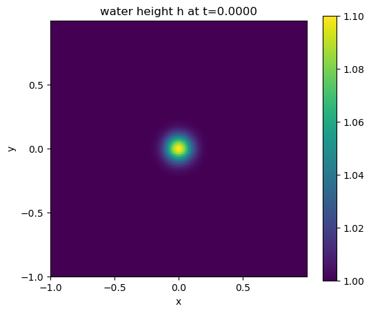
The hump collapses and sends out a circular wave. At \( t=0.2\) , the wave crest has travelled around 0.68 from the centre. This matches the wave speed \( \sqrt{gh} \approx 3.13\) . Behind the crest, the water level drops below 1:
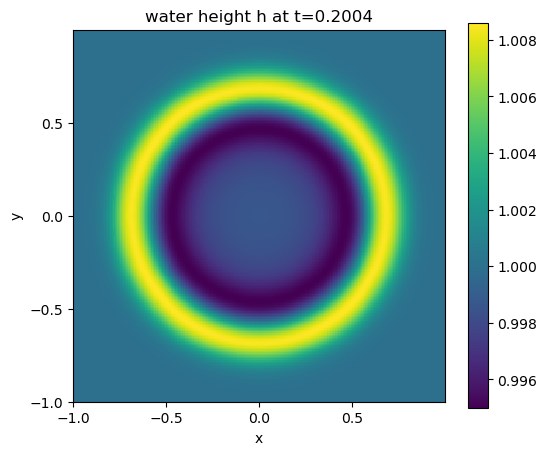
At around \( t=0.3\) , the wave reaches the boundary of the domain. As the domain is periodic, it re-enters from the opposite side, and the waves from the four sides meet in the corners:
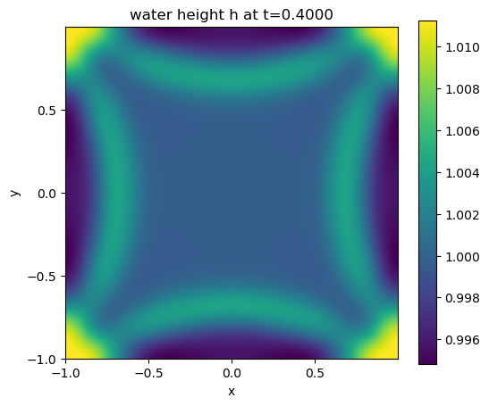
The total amount of water is conserved exactly. You can check this by summing up h over all volumes of any snapshot.
The pictures are created by tutorials/exahype2/illustrations/11_tsunami.py, which runs exactly this setup.
Writing the flux by hand is error-prone. We have to translate each entry of the flux matrix into C++, and the eigenvalues have to be worked out on paper first. SymPy, Python's library for symbolic mathematics, can do both jobs for us: we write down the flux matrix as it stands in the formula at the top, let SymPy derive the eigenvalues, and let SymPy print the C++ code. The result is a string again, which we inject exactly as before.
We run through exactly the same steps as above, but use a new project directory 11_tsunami-sympy, so the two versions do not overwrite each other.
We introduce one symbol per unknown plus the gravity \( g\) . Telling SymPy that \( h\) and \( g\) are positive allows it to simplify \( \sqrt{g h}\) later on. Column \( n\) of F is the flux in direction \( n\) :
The eigenvalues of the flux's Jacobian \( \partial F_n / \partial Q\) tell us how fast information travels in direction \( n\) . We no longer have to work them out on paper:
SymPy confirms the eigenvalues \( u_n - \sqrt{gh}\) , \( u_n\) and \( u_n + \sqrt{gh}\) from the beginning of this tutorial, with \( u_n = hu_n/h\) . The Rusanov scheme needs the biggest absolute value of these eigenvalues.
sympy.cxxcode() turns an expression into C++. With assign_to, it writes a whole assignment. We wrap the generated assignments into a small prologue which defines g and reads the unknowns from Q via their symbolic names. As the flux and the eigenvalue differ per direction, we generate one branch per normal:
This code is less compact than our handwritten version, but we did not write a single line of it. We inject it exactly as before. We keep the initial condition handwritten.
Numerical scheme, mesh, plotter and global parameters are the same as before:
The two codes should give the same solution, even though SymPy arranges the arithmetic differently, e.g. it writes std::pow(h, 2) where we wrote h * h. We read the last snapshot of both runs and compare the water height:
SymPy reproduces our handwritten physics: the two solutions agree in all digits that the output files hold. These files store six significant digits per value. Tiny round-off differences, as floating-point operations in a different order may round differently, would therefore not show up here. The pictures from above therefore hold for this version, too.
So far, the water depth is 1 everywhere: the sea floor is flat with \( b=0\) , and the water stands at \( h=1\) besides the hump. Real oceans are not flat. We therefore now give the basin a sea floor with some structure: the water is 4 deep where the logo of Durham University is purple, and 1 deep where it is white.
The depth enters the setup twice. The water column \( h\) starts at the local depth, and the sea floor sits at \( b=-\text{depth}\) , so the water surface \( h+b\) is flat besides the hump.
The logo is an image of \( 200 \times 200\) pixels. Injecting 40,000 pixels as a Python string would be awkward. Instead, the depth map lives in two C++ files next to this notebook, which we add to the build: bathymetry/DurhamLogo.h declares an array DurhamLogo with one string per row of pixels, starting with the top row. A 1 in a string marks a purple pixel. bathymetry/DurhamLogo.cpp holds the actual data.
The two files are part of the repository, so the tutorial does not need internet access. They were created once by bathymetry/create-durham-logo.py, which downloads the logo and translates its pixels into C++. Whenever you have data such as a real bathymetry, it is often simplest to translate it into C++ in a similar way.
We set up the solver exactly as before. The only additional thing is that the solver has to include the header:
The initialisation looks up the pixel which covers x and sets the depth accordingly. The image's top row covers \( y=1\) . Flux and eigenvalue are the ones that we derived with SymPy:
b is an auxiliary variable, which we also call a material parameter. ExaHyPE stores it with each degree of freedom, i.e. each finite volume holds its own copy of b right after the unknowns in Q. It is handed to every PDE term, it is written into the output files, and it travels with the volume when the mesh changes or is distributed between ranks.
However, the hyperbolic kernels do not evolve it. A time step updates the unknowns h, hu and hv. b is copied over unaltered. If b should change over time, e.g. as a quake lifts the sea floor, you can overwrite it on-the-fly: b is an ordinary entry of Q, so any of your routines which writes into Q may change it. From thereon, the kernels carry the new value along.
ExaHyPE lowers its project into a Peano project. Before we let the Peano project generate its code, we tell its makefile about our additional files: the implementation file has to be compiled and linked, and the compiler has to find the header. All paths are relative to the directory of the generated code.
Switch the viewer to b to see the sea floor, and to h to see the water:
Our sea floor is the logo, 3 lower where the logo is purple:
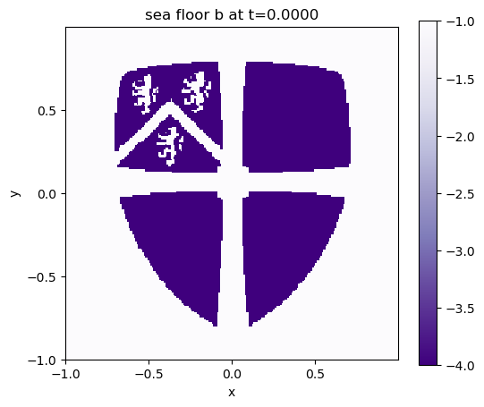
At \( t=0\) , the water surface \( h+b\) is flat besides the hump. The water column \( h\) however is 3 higher above the purple parts:
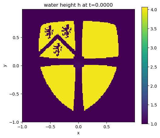
And then the logo falls apart. Each edge of the logo behaves like a small dam which breaks:
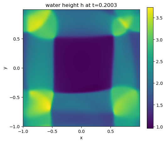
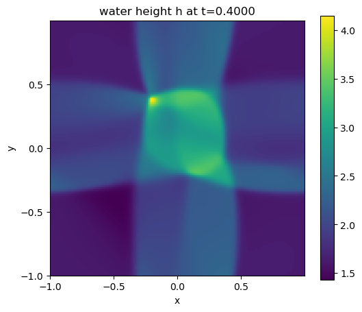
This is not what a real ocean does. Water at rest above a deep trench stays at rest. Our PDE terms however never read b: they see a water column which is higher in some places than in others, and let it flow. The sea floor only shapes the flow once the term \( g h \nabla b\) enters the equations. We add it in the next step.
What did happen is that b did not change at all. We compare the first and the last snapshot:
The pictures are created by tutorials/exahype2/illustrations/11_tsunami.py, too.
In the previous section, the sea floor was carried along, but it did not enter the PDE. We now bring in the missing term \( g h \nabla b\) . ExaHyPE solves PDEs of the form
\begin{eqnarray*} \frac{\partial Q}{\partial t} + \nabla \cdot F(Q) + B(Q) \nabla Q = 0, \end{eqnarray*}
where \( B(Q) \nabla Q\) is the non-conservative product. We cannot write \( g h \nabla b\) as the divergence of a flux, as b may jump, and the gradient of a jump does not exist. As a non-conservative product, it is fine: the kernels hand over the jump of Q over each face of a volume rather than a gradient, and we return \( B(Q)\) times this jump. In our case, \( B\) maps the jump of b in direction normal onto \( g h\) times this jump in the momentum equation of the same direction.
The water again starts at rest, and the only disturbance is the very same point tsunami that we used in the first part of this tutorial. The bathymetry can only show its impact over time, as the tsunami spreads.
There is one catch. The Rusanov scheme adds numerical dissipation which is proportional to the jumps of the unknowns between neighbouring volumes. If we keep h as unknown, the water at rest is 4 deep above the purple and 1 deep above the white parts of the logo. The scheme sees a jump in h at each edge of the logo, dissipates it, and the water starts to flow although it should rest.
We therefore switch to the surface elevation \( \eta = h + b\) as unknown. Water at rest has a flat surface, i.e. a constant \( \eta\) , and the scheme sees no jump whatsoever. Within the PDE terms, we reconstruct the water height as \( h = \eta - b\) . This way, the bathymetry enters the flux and the eigenvalues, too. For Rusanov's averaging of the flux and the non-conservative product, one can show that the two then cancel out exactly for water at rest.
As \( b\) does not change over time, \( \partial_t \eta = \partial_t h\) , i.e. we solve the same equations.
We take the flux matrix and the eigenvalues from the SymPy section and replace h by \( \eta - b\) :
The non-conservative product is short enough to write it by hand. Q is the average of the two volumes adjacent to a face, deltaQ the jump between them. Both hold the unknowns and the auxiliary variables, so we can read the jump of b:
The initial condition is the one from the previous section, but written in terms of \( \eta\) : the surface is flat besides the hump, i.e. \( \eta\) holds only the point tsunami, and the water does not move.
Everything else is the same as in the previous section, including the external files:
At \( t=0\) , the surface is flat besides the hump in the centre, and nothing hints at the logo underneath:
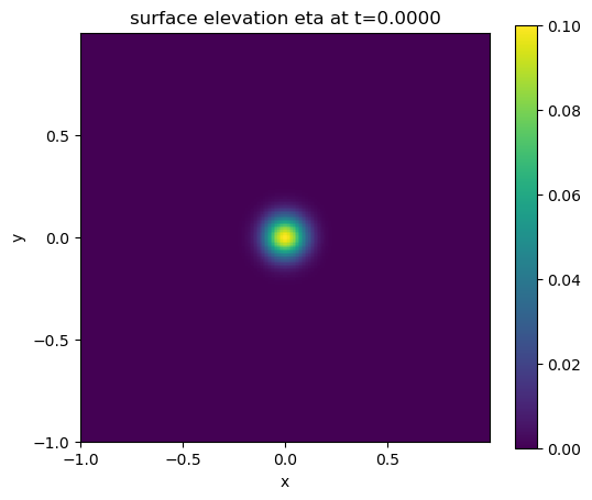
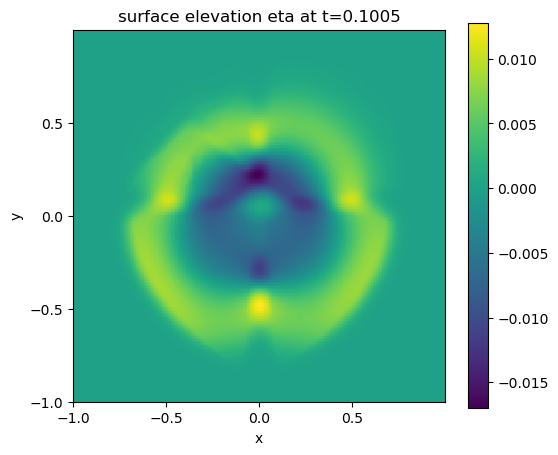
Away from the wave, the water stays at rest. The logo does not fall apart anymore. However, the wave now feels the sea floor. Its speed is \( \sqrt{g h}\) , i.e. around 6.26 above the purple parts of the logo, where the water is 4 deep, and only 3.13 above the white parts. Over the flat sea floor of the first part, the wave crest is around 0.36 away from the centre at \( t=0.1\) , in all directions. Over the logo, it has run around 0.66 into the two lower quarters of the shield, which are deep everywhere. Towards the two upper quarters, it is only at around 0.51 to 0.55, as the wave first has to cross the shallow, horizontal bar of the white cross. Along the vertical bar of the cross, the wave lags behind most: its crest is at 0.44 upwards and 0.49 downwards. There, the wave also is higher than elsewhere, as a wave which slows down piles up:
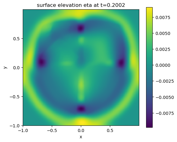
At \( t=0.2\) , the wave has crossed most of the basin, and the white cross is imprinted on it:
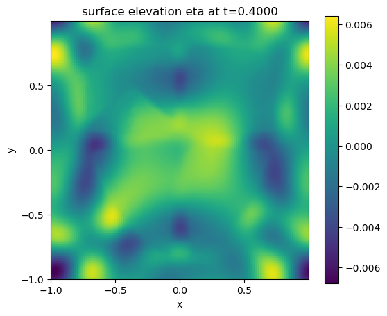
Once the waves re-enter through the periodic boundaries, they overlap with waves which took different routes over the logo, and the pattern becomes complex:
The pictures are created by tutorials/exahype2/illustrations/11_tsunami.py, too.
 1.9.8