 |
Peano
|
|
Peano
|
So far, all solvers in our tutorials have been active everywhere: Each solver holds its data in every (unrefined) cell of the mesh, and it updates these data in each and every time step. Localisation is the opposite: A solver is active only in a part of the mesh, i.e. it neither stores nor updates any data elsewhere. Localisation comes in two flavours:
We start with the motivation for the latter flavour, before we discuss the mechanics of localisation along the lines of the former. As soon as solvers are localised, they typically have to exchange data where their active regions meet or overlap. This is discussed in Coupling of various solvers.
Localisation in resolution might look like an exotic feature, but it is a key ingredient of many modern uncertainty quantification (UQ) methods. In UQ, we do not run one simulation, but many: We are interested in the statistics of some output quantity \( Q\) , such as the expected wave height at a buoy, where the input data (initial conditions, material parameters, bathymetry, ...) are uncertain. A plain Monte Carlo estimate averages \( Q\) over \( N\) samples. Its statistical error decays with \( N^{-1/2}\) only, so we need many samples, and each sample is a full PDE solve on a fine mesh. This quickly becomes prohibitively expensive.
Multilevel Monte Carlo (MLMC) (Giles 2008; Giles 2015) reduces this cost by exploiting a hierarchy of meshes \( \ell = 0, 1, \ldots, L\) from coarse to fine. It rewrites the expectation on the finest mesh as a telescoping sum
\begin{eqnarray*} \mathbb{E}[Q_L] = \mathbb{E}[Q_0] + \sum_{\ell=1}^{L} \mathbb{E}[Q_\ell - Q_{\ell-1}] \end{eqnarray*}
and estimates each term with its own number of samples. Most samples are taken on the cheap coarse meshes. The corrections \( Q_\ell - Q_{\ell-1}\) have a small variance and hence need only a few of the expensive fine-mesh samples. Mishra, Schwab and Šukys (2012) have shown that this pays off for nonlinear hyperbolic systems of conservation laws such as the Euler or the shallow water equations, i.e. for exactly the type of problems that ExaHyPE is written for. Multi-index Monte Carlo (Haji-Ali, Nobile and Tempone 2016) generalises the idea to several hierarchies at once, such as the mesh size and the time step size.
The same idea carries over to Bayesian inverse problems, where we infer uncertain parameters from measurements through Markov chain Monte Carlo (MCMC): Multilevel MCMC (Dodwell et al. 2015) and multilevel delayed acceptance (Lykkegaard et al. 2023) use cheap coarse-mesh solves to steer or screen proposals before the expensive fine-mesh solve is invoked. Seelinger et al. (2021) have parallelised multilevel MCMC on supercomputers and identified the source of a tsunami from buoy data, using ExaHyPE (Reinarz et al. 2020) as forward solver. All of these approaches belong to the wider family of multi-fidelity methods (Peherstorfer, Willcox and Gunzburger 2018), which combine cheap low-fidelity models with expensive high-fidelity ones.
Where does localisation come into play? The crucial term in the telescoping sum is the correction \( Q_\ell - Q_{\ell-1}\) : Both \( Q_\ell\) and \( Q_{\ell-1}\) have to be computed for the very same sample, i.e. with the very same uncertain input. Otherwise, the two do not correlate, and the variance of their difference is not small. Typical UQ codes realise this through two independent simulations, one per mesh, and they have to ensure that both see the same input. With localisation in resolution, we can realise both simulations within one mesh instead: One solver instance lives on level \( \ell\) of the spacetree, the other one on level \( \ell-1\) . Two adjacent levels of Peano's spacetree differ by a factor of three in the mesh size, which yields a natural level hierarchy. Both solvers share the mesh, the input data, the parallelisation and the domain decomposition, and their difference can be computed on-the-fly, cell by cell, rather than in a postprocessing step. The same reasoning holds for the pairs of coarse and fine models within multilevel MCMC.
We now realise the idea behind the telescoping sum within one simulation: We take the Euler equations from A first advection problem with the Euler equations and solve them twice within the same mesh. One solver, EulerFV, runs on a fine mesh. A second solver, CoarseEuler, uses exactly the same routines, but it lives on one coarse level of the spacetree only. Both see the very same initial condition, i.e. their outputs correspond to \( Q_\ell\) and \( Q_{\ell-1}\) for one sample.
The fine solver is the solver from A first advection problem with the Euler equations. We only ask for smaller volumes, i.e. a finer mesh:
The second solver needs a flux, an eigenvalue and an initial condition, too, and they should be the very same ones. We could copy EulerFV's implementation file, but then we would maintain two copies of the same physics. Instead, we let CoarseEuler forward each call to EulerFV.
ExaHyPE creates one global instance per solver, which lives in the namespace repositories of our project: repositories::instanceOfEulerFV is the fine solver object. As we inject all PDE terms of CoarseEuler, ExaHyPE does not generate a class CoarseEuler for us to fill. The injected code ends up in the implementation file AbstractCoarseEuler.cpp, and so do the solver includes. Therefore, we can include the solver repository there without creating a cyclic include:
Each solver holds a grid selector. The selector decides on which vertices, faces and cells all of the solver's action sets act, and where Peano stores the solver's data. By default, a solver uses a FineGridSelector, i.e. it works on the finest mesh level only.
CoarseEuler gets a FixedResolutionGridSelector instead. It selects all mesh entities of one level of the spacetree, no matter whether the mesh is refined further there or not. Level 0 is the root of the spacetree, i.e. the whole domain, and each level splits its cells into \( 3 \times 3\) children. Level 2 hence consists of \( 9 \times 9\) cells, and with patches of \( 9 \times 9\) volumes, CoarseEuler works on \( 81 \times 81\) volumes. The fine solver asked for volumes of size 0.001, so ExaHyPE refines the mesh down to level 3. EulerFV hence works on \( 243 \times 243\) volumes.
Both solvers construct a regular grid. CoarseEuler's grid construction asks for level 2 only, EulerFV's for level 3. The mesh is the union of the two, i.e. it is refined down to level 3 everywhere, and each solver picks its level through its selector.
The remaining steps are the same as in A first advection problem with the Euler equations. We add both solvers to the project, and we write the implementation of EulerFV.
There is a class EulerFV for us to implement, but no class CoarseEuler. We fill EulerFV.cpp with the implementation from A first advection problem with the Euler equations, i.e. the code which CoarseEuler forwards to:
Each solver has its own plotter, so we get two sets of patch files: solution-EulerFV and solution-CoarseEuler. Each solver decides on its own when to plot, i.e. it plots as soon as its own time stamp has passed the next plot time. The snapshots of the two solvers therefore carry slightly different time stamps:
You can open both files in the notebook viewer, or convert both into VTK and load both pvd files into Paraview. CoarseEuler's patches are three times as big as EulerFV's patches, and they cover the same domain. Show one at a time, or shrink or shift one of them to see both.
As the snapshots do not match exactly in time, we compare the two solvers in two ways that cope with this.
First, we probe both solvers at the same point. Each probe yields a time series with its own time axis, so we can plot the two series over each other without pairing up snapshots:
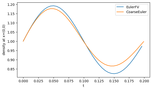
The coarse solver's wave has a smaller amplitude. Furthermore, EulerFV's curve ends a little earlier: the run stops once CoarseEuler has reached \( t=0.2\) .
Second, we compare whole snapshots. We pair each snapshot of one solver with the snapshot of the other solver which is closest in time, and plot the two with the same colour range:
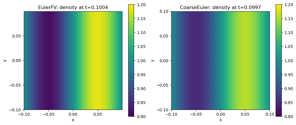
Both solvers advect the same density wave. The coarse solver however smears it out more: Rusanov's numerical diffusion scales with the size of the volumes. At \( t=0.2\) , the coarse density ranges from around 0.88 to 1.12, whereas the fine solver still yields around 0.83 to 1.17. The initial condition oscillates between 0.8 and 1.2.
The pictures are created by tutorials/exahype2/illustrations/44_localisation.py.
This subsection describes ideas only. None of them is implemented yet, i.e. the code above behaves as described in the note, not as sketched here.**
Today, each solver computes its time step size from the CFL condition with its own maximum eigenvalue, but with the smallest volume of the whole mesh: The action set ComputeGlobalCFLCondition takes the mesh size from Peano's grid statistics, which know nothing about solvers or grid selectors. CoarseEuler therefore marches with time steps that fit EulerFV's volumes, although its own volumes are three times as big.
The idea is to let each solver use the size of its own volumes instead, reduced the same way as the maximum eigenvalue already is:
With this change, CoarseEuler would take time steps roughly three times as big as EulerFV's, and it would reach the end time after roughly a third of the time steps. As the simulation terminates as soon as the first solver reaches the end time, EulerFV would stop at around \( t \approx 0.07\) . A second idea addresses this: The main loop could run until every solver has reached the end time. Each solver already shortens its last time step such that it does not overshoot the end time, i.e. a solver which is done would simply idle with time step size 0 until the others have caught up. Alternatively, the solvers could agree on one common time step size. Which option is the right one depends on whether the solvers exchange data, which is what the text part of this tutorial discusses.
ExaHyPE couples volumetrically. That does not mean that all solvers have to be solved everywhere. Indeed, the idea to offer support for multiple solvers arose originally from the a posteriori limiting of Dumbser et al where a Finite Volume solver complements ADER-DG solutions where shocks arise.
Most projects that follow these rationale realise the same pattern: We define two different solvers, and we couple them with each other. The coupling (and solve) however are local operations:
We will effectively end up with a domain decomposition where parts of the computational domain are handled by the higher-order solver and the other parts are handled with FV. To realise this, we need a marker or oracle, i.e. a magic function per cell which tells us, similar to a multi-phase flow, which solver rules in this particular cell. The marker will guide us which solver is "valid" in which cell, where one solver overrules the other one, and where we do not have to store one solver's data or the other.
The image below illustrates the core idea behind typically coupling approaches in ExaHyPE. The sizes of the overlap might differ, but the principle is always the same. The illustration shows the minimal overlap that we can typically use. Both the upper and the lower mesh illustrate the same mesh. I use colours to show which solver exists in which mesh cell.
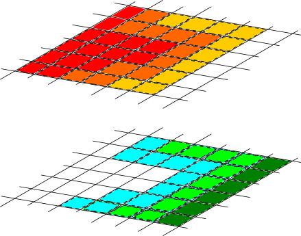
Starting from this description, sophisticated coupling equations can be realised, where you exploit the fact that we have a volumetric overlap.
Skip this section if you prefer a hard-coded marking of active regions.
Once you know where a solver is valid, it makes sense also to only store the solver's data in the valid region. Otherwise, a lot of memory is "wasted" which furthermore will be moved/accessed in each and every grid sweep, as the mesh management of Peano so far does not know that ExaHyPE might not need the data. ExaHyPE has to let Peano know.
The technical principles behind such a localisation are discussed in a Peano tutorial of its own. ExaHyPE builds up pretty deep inheritance hierarchy where every subclass specialises and augments the basic numerical scheme, and also implements additional guards when data is stored or not. However, most of these subclasses rely on only six routines to control the data flow:
The implementation then uses these predicates to puzzle the actual storage scheme together via calls similar to
By default, most solvers only store data for unrefined cells. They mask coarser levels with in the tree out. Subclasses such as enclave tasking variations augment the guards further such that not all data are stored all the time. Nothing stops you from adding further constraints and to use a solver only in a certain subdomain for example.
 1.9.8