 |
Peano
|
|
Peano
|
This standard test case is used to assess the adaptive mesh refinement and to illustrate the importance of a symplectic time integrator.
The setup simulates the Earth rotating around the Sun. So we actually have only one (free) particle with a hard-coded force function. The realisation is subject of a tutorial session which demonstrates how to inject user-defined force functions into the default Euler and leapfrog ODE integrators.
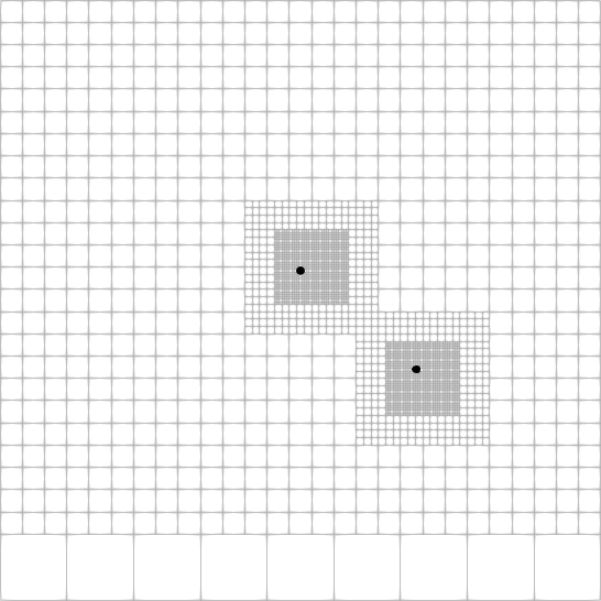
Usage is relatively straightforward
The code spills out a series of vtu files for the particles including one pvd file that serves as overview/meta file. You can load this one straight into Paraview, e.g. The grid visualisation requires a separate postprocessing step before you can visualise it as native file. Please note that the snippet above uses an explicit Euler which is not capable to reproduce a stationary orbit, as it is a non-symplectic time integrator.
Depending on the mesh size, you get different AMR levels. I extract them into a table below, but it actually makes more sense to study the README-orbit-xxx.md file that the Python script produces. It provides all the essential information per experiment.
| Cell size | Levels | Remarks |
|---|---|---|
| 0.4 | 0 | Regular 81x81 mesh. No dynamic adaptivity (default). |
| 0.1 | 1 | Around 234 mesh cells with one level of adaptivity. |
| 0.03 | 2 | Two levels of adaptivity. The number of mesh cells starts to change almost every time step. |
| 0.01 | 3 | More radical version with three levels of adaptive mesh refinement. |
ExaParty's AMR analysis works on a per-cell basis. For each cell, it studies all four adjacent vertices, and sums up the number of particles stored there. As we set the maximum number of particles to 0, every cell that is adjacent to a vertex holding the single particle will issue a refine command
To run the test, you can either follow the instructions below one by one (which allows you to tailor some settings), or you run the ./run.sh script from the test's directory. This script will automatically invoke the postprocessing, too. Please note that the run script builds the executables in assert mode, i.e. it ensures that there are no runtime errors.
I recommend to use the Python Paraview variant to convert the arising mesh files into something you can visualise straightforwardly.
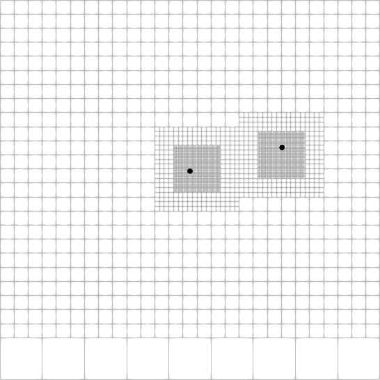
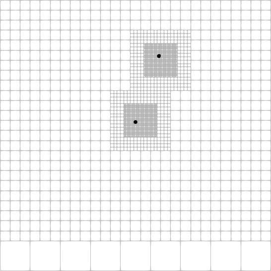
The test is supplemented with a Python script which assesses the energy conservation and yields some overview plots. The script assumes that you did dump some output data into the current directory.
python3 ./plots-time-integration-test.py
It should create some global stats as well as a plot of the energy over time:
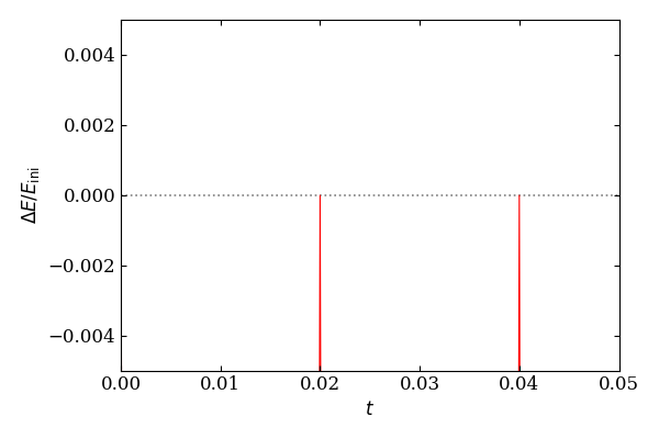
Please note that the script currently works only for a serial run. The plot above stems from a parallel experiment and hence shows a lot of gaps.
The instruction snippets below clean up the majority of the file spilled out by this benchmark. All files that are essential to rerun the benchmark and are stored in the repo are kept:
 1.9.8