This simple tutorial runs through the steps that we followed to create the planet orbit test case, which basically ensures that the AMR underlying ExaParty works.

High-level code structure

We need Peano's core Python package, the ExaParty package, and then we employ DaStGen 2 which is a tool that allows Peano to write plain C++ classes which hold our particle data, e.g. We will add additional attributes to this data set and hence use the DaStGen2 package.

Create project

First of all, we have to create a project. The project is our wrapper of the whole SPH code (which is not really SPH but simply a simple Lagrangian model for an object subject to an ODE):

project = exaparty.api.Project(
    namespace=["tests", "exaparty", "planetorbit"],
    project_name="planetorbit",
    executable="orbit-" + str(args.cell_size),
)

This snippet stems from tests/exaparty/planet-orbit/planet-orbit.py.

Configure the overall simulation

Peano will need to know the value of some general properties. For more information, consult the documentation of exaparty.api.Project and also the remarks on build variants:

if args.asserts:
    build_mode = peano4.api.output.CompileMode.ASSERTS
else:
    build_mode = peano4.api.output.CompileMode.RELEASE
 
offset = [0, 0, 0]
domain_size = [1, 1, 1]
periodic_boundary_conditions = [False, False, False]  # Periodic BC
 
project.set_global_simulation_parameters(
    dimensions=dimensions,
    offset=offset,
    domain_size=domain_size,
    min_end_time=args.end_time,
    max_end_time=0.0,
    first_plot_time_stamp=0.0,
    time_in_between_plots=args.plot_delta,
    periodic_BC=periodic_boundary_conditions,
    plotter_precision=8,  # plotter precision
)
 
project.set_load_balancing(
    "toolbox::loadbalancing::strategies::SpreadOutHierarchically",
    "new toolbox::loadbalancing::DefaultConfiguration()",
)
 
project.set_Peano4_installation(args.peanodir, build_mode)

The call of exaparty.api.Project.set_load_balancing() activates one of Peano's generic load balancing strategies. The last line is notably interesting: It instructs the Python API to parse the settings of your configure (autotools) or CMake run. That is, all the flags that you specified throughout your installation will automatically be picked up by the code that the Python script will ultimately produce.

Generate a genuine Peano project

Once all is complete, we generate a Peano project and make it dump the C++ code:

481peano4_project = project.generate_Peano4_project(verbose=args.verbose)

After the project is generated, we add the compile constants required (see below) and then can dump it into the file system and either compile it in place through the Python script, or leave it to the user to type in make.

Particle implementation

Instantiate particle (and select species)

A particle in ExaParty is defined by its type which implicitly select its numerics. Once instantiated, we say the particle has a species. In this simple example, we don't really have an interaction radius, so we can take the simplest particle with a fixed interaction radius.

We need a leapfrog time integrator rather than an explicit Euler to maintain a stable radius. However, we can provide various different schemes and just swap them in an out.

Besides the time stepping scheme (which implicitly defines the steps any particle completes per time step), each particle guides the size of the underlying adaptive mesh. We therefore specify min_h and max_h.

    particle = exaparty.api.particle.LeapfrogFixedSearchRadius(
        name="Planet",
        cfl_factor=0.2,
        initial_time_step_size=args.timestep_size,
        particles_per_cell=0,
        min_h=args.cell_size,
        max_h=0.3,
    )
    particle_set = project.add_particle_species(particle)

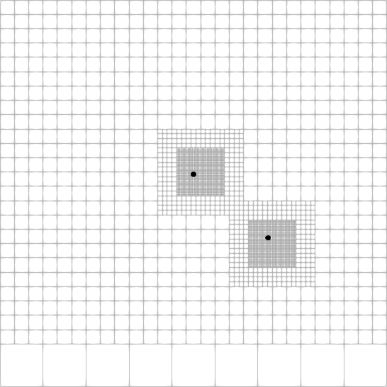
As we set the interaction radius to zero later on, and as we set the particles_per_cell to zero, the code will run into a dilemma: There will always be one cell in the mesh which hosts one particle which violates the zero threshold. So the code will aggressively refine until the mesh is smaller than min_h. That stops the refinement no matter of the violated particles_pre_cell constraint.

Adding additional attributes

So far, our particles are primitive. They will hold a position and a maximum search radius, as any particle within Peano's particle toolbox owns these properties. The integration of choice will add further attributes. In the present case, that's speed and acceleration. But other than that, the particle so far has no properties. We add a few ones:

energy_kin_attr = dastgen2.attributes.Double("energyKin")
energy_pot_attr = dastgen2.attributes.Double("energyPot")
energy_tot_attr = dastgen2.attributes.Double("energyTot")
particle.data.add_attribute(energy_kin_attr)
particle.data.add_attribute(energy_pot_attr)
particle.data.add_attribute(energy_tot_attr)

The package dastgen2.attributes hosts also arrays of doubles and integers and booleans. Please note that there is an opportunity to specify accuracies (valid bits) for floating point values and upper and lower bounds for integers. Such additional information allows Peano in combination with our LLVM modifications to produce particularly memory-efficient code.

Injecting the physics

We start with the definition of some constants.

# Orbital parameters
N_orbits = 8
# Number of orbits
G_NEWTON = 6.67384e-11
# Newton's constant  [m^3/kg/s^2]
M_SUN = 1.9885e30
# Sun mass [kg]
M_EARTH = 5.97219e24
# Earth mass [kg]
R_MAX = 152097701000.0
# [m]
R_MIN = 147098074000.0
# [m]
V_MAX = 30287.0
# [m/s]
 
# Initial positions in internal units
LENGTH_UNIT = 4.0 * R_MAX
SUN_X_COORD = str(0.5)
SUN_Y_COORD = str(0.5)
EARTH_X_INI = str(float(SUN_X_COORD) + R_MAX / LENGTH_UNIT)
EARTH_Y_INI = SUN_Y_COORD
 
# Derived quantities
e = (R_MAX - R_MIN) / (R_MAX + R_MIN)
# Eccentricity [dimensionless]
b = np.sqrt(R_MAX * R_MIN)
# Semi-minor axis [m]
p = b * np.sqrt(1.0 - e * e)
# Semi-lactus rectum [m]
a = p / (1.0 - e * e)
# Semi-major axis [m]
T = np.sqrt(4.0 * np.pi * np.pi * a * a * a / (G_NEWTON * (M_SUN + M_EARTH)))
# Period [s] */
 
# Time-step size
dt = 1e-3 * T
# [s]
dt /= T
N = N_orbits / dt
GLOBAL_TIME_STEP_SIZE = str(dt)
 
# Initial velocity in internal units
EARTH_V_INI_X = str(0.0)
EARTH_V_INI_Y = str(V_MAX / LENGTH_UNIT * T)

The actual export happens later:

 
# Export symbols and values for compilation (e.g. for SPH kernel)
# Dummy values for non SPH
peano4_project.output.makefile.add_CXX_flag("-D" + "HYDRO_DIMENSION=1")
peano4_project.output.makefile.add_CXX_flag("-D" + "HYDRO_GAMMA_5_3")
peano4_project.output.makefile.add_CXX_flag("-D" + "QUARTIC_SPLINE_KERNEL")
 
peano4_project.constants.export_const_with_type(
    "GLOBAL_TIME_STEP_SIZE", GLOBAL_TIME_STEP_SIZE, "double"
)
peano4_project.constants.export_const_with_type("G_NEWTON", str(G_NEWTON), "double")
peano4_project.constants.export_const_with_type(
    "LENGTH_UNIT", str(LENGTH_UNIT), "double"
)
peano4_project.constants.export_const_with_type("M_SUN", str(M_SUN), "double")
peano4_project.constants.export_const_with_type("SUN_X_COORD", SUN_X_COORD, "double")
peano4_project.constants.export_const_with_type("SUN_Y_COORD", SUN_Y_COORD, "double")
peano4_project.constants.export_const_with_type("EARTH_X_INI", EARTH_X_INI, "double")
peano4_project.constants.export_const_with_type("EARTH_Y_INI", EARTH_Y_INI, "double")
peano4_project.constants.export_const_with_type(
    "EARTH_V_INI_X", EARTH_V_INI_X, "double"
)
peano4_project.constants.export_const_with_type(
    "EARTH_V_INI_Y", EARTH_V_INI_Y, "double"
)
peano4_project.constants.export_const_with_type("ECCENTRICITY", str(e), "double")
peano4_project.constants.export_const_with_type("PERIOD", str(T), "double")
peano4_project.constants.export_const_with_type("R_MIN", str(R_MIN), "double")
peano4_project.constants.export_const_with_type("R_MAX", str(R_MAX), "double")

Add the forces

To add the forces, we have attach a C/C++ code snippet to the particle. In our present case, the force is hard-coded, i.e. does not depend on other particles. It uses some constants that we have previously defined in the Python script. Here, we have now two options:

We can take the C++ code snippet in Python and replace the constant strings in there via a Python format() call. The C++ code then will see the actual constants as hard-coded values.
We can use some constants like SUN_X_COORD in the C++ code and define these as proper constants in the generated C++ code.

In the example below, we go down the second route. That means, the code as it stands will contain some constants like SUN_X_COORD. We have to ensure that these constants are properly exported into the Peano project. Both approaches (replacing literals before we dump the code snippet into the Python API and defining C++ constants) are fine and work. It is all a matter of taste.

 
particle_force = """
// Template in tests/exaparty/planet-orbit.py
 
::exaparty::kernels::forAllParticles(
  marker,
  localParticles,
  numberOfCoalescedLocalParticlesPerVertex,
  [=](
    const peano4::datamanagement::CellMarker& marker,
    globaldata::Planet&                       localParticle
  ) -> void {
    if ( ::exaparty::kernels::localParticleCanBeUpdatedInCellKernel(
      marker,
      localParticle
    )) {
      #if Dimensions==2
      tarch::la::Vector<Dimensions,double> pos_sun = {SUN_X_COORD,SUN_Y_COORD};
      #else
      tarch::la::Vector<Dimensions,double> pos_sun = {SUN_X_COORD,SUN_Y_COORD,0.0};
      #endif
 
       /* G_NEWTON in internal units */
      double const L3 = LENGTH_UNIT * LENGTH_UNIT * LENGTH_UNIT;
      double const T2 = PERIOD * PERIOD;
      double const GN = G_NEWTON * M_SUN * T2 / L3;
      //double GN = 1.0;
 
      tarch::la::Vector<Dimensions,double> earthSunDistance = localParticle.getX() - pos_sun;
      const double r = tarch::la::norm2(earthSunDistance);
      if (tarch::la::greater(r,0.0)) {
        const double r_inv =  1.0 / r;
        localParticle.setA( - GN * earthSunDistance * (r_inv * r_inv * r_inv) );
 
        /* Update Energy */
        const double vel = tarch::la::norm2( localParticle.getV() );
        const double E_kin = 0.5 * vel * vel;
        const double E_pot = - GN * r_inv;
 
        /* Update total energy (overall minus sign) */
        localParticle.setEnergyKin( E_kin );
        localParticle.setEnergyPot(-E_pot );
        localParticle.setEnergyTot( - ( E_kin + E_pot ) );
      } // end of radius check
    } // end of "may I update" check
  }, // end of functor
  ::exaparty::kernels::alwaysUpdateInCellKernel<globaldata::Planet>
);
 
// end template
"""
 
particle.cell_kernel = particle_force

The code now is fully functional, but will not produced any output, as we haven't inserted any particle into our computational domain yet. Even if we do so, we will only see the particles and not their properties, as the code knows nothing about these properties. Please study the script benchmarks/exaparty/planet-orbit/planet-orbit.py for more documentation how these two missing steps are to be realised.

If we had some proper n-body physics, we would use another iterator, i.e. one that runs through the particle pairs.

Set initial conditions

 
search_radius = args.cell_size / 100.0
initialisation_snippet = (
    """
  /*
   * In this problem we will initialize just a single particle (Earth)
   * This will orbit around a point where the hypothetical Sun is (no particle needed here)
   */
 
  /* Internal search radius used by Peano.
   * Should always be larger than actual SPH interaction radius (~2h).
   * But no really used here. */
  particle->setSearchRadius("""
    + str(search_radius)
    + """);
  particle->setV( {0, 0, 0} );
  particle->setA( {0, 0, 0} );
 
  // Orbiting particle: We can also have a free moving sun, but by default, this
  // one rests and the earth is actually orbiting.
  if( particle->getX(0) == EARTH_X_INI ){
    particle->setV(0, EARTH_V_INI_X) ;
    particle->setV(1, EARTH_V_INI_Y) ;
  }
 
  /*
   * Set initial energy
   */
 
  /* G_NEWTON in internal units */
  double const L3 = LENGTH_UNIT * LENGTH_UNIT * LENGTH_UNIT;
  double const T2 = PERIOD * PERIOD;
  double const GN = G_NEWTON * M_SUN * T2 / L3;
 
  /* Sun-Earth initial distance */
  const double r_ini = particle->getX()(0) - SUN_X_COORD;
  const double r_inv = r_ini ? 1.0 / r_ini : 0.0;
  const double vel = tarch::la::norm2( particle->getV() );
 
  const double E_kin = 0.5 * vel * vel;
  const double E_pot = - GN * r_inv;
 
  particle->setEnergyKin( E_kin );
  particle->setEnergyPot(-E_pot );
 
  /* Overall minus sign for plotting */
  particle->setEnergyTot( -( E_kin + E_pot ) );
 
  logInfo( "Init()", "=====================================" );
  logInfo( "Init()", "Initial energy:");
  logInfo( "Init()", "Kinetic energy  :" << E_kin);
  logInfo( "Init()", "Potential energy:" << E_pot);
  logInfo( "Init()", "Total energy    :" << E_kin + E_pot);
  logInfo( "Init()", "Search Radius   :" << particle->getSearchRadius() );
  logInfo( "Init()", "Initial velocity:" << particle->getV() );
  logInfo( "Init()", "=====================================" );
 
 
"""
)
 
#
# Insert Earth into system
#
project.algorithm_step_initial_conditions.add_action_set(
    exaparty.api.input.InsertParticlesByCoordinates(
        particle_set=particle_set,
        initialisation_call=initialisation_snippet,
        coordinates=[(EARTH_X_INI, EARTH_Y_INI, 0)],
    )
)

Plot

 
particle_plotter = peano4.api.toolbox.particles.PlotParticlesInVTKFormat(
    "particles",
    particle_set,
    "globaldata::{}::getSpecies().getMinTimeStamp()".format(particle.name),
)
particle_plotter.add_attribute_to_plot(particle.velocity, dimensions)
particle_plotter.add_attribute_to_plot(energy_kin_attr, 1)
particle_plotter.add_attribute_to_plot(energy_pot_attr, 1)
particle_plotter.add_attribute_to_plot(energy_tot_attr, 1)
project.algorithm_step_plot.add_action_set(particle_plotter)

A better code structure

The code above is fully functional. One however might argue that the mixture of Python code and string-based C++ code is not particularly nice, hardly reusable and difficult to debug: You have to generate the code, compile, parse the error and then reconstruct where in the Python script it comes from. It hence would be nicer to define the Physics in a header/implementation file of its own. Once we have a Peano project in Python, we can add further C++ files to its make file. That is, we can implement the Physics independently and then add these files to the project manually. This way, we work with Python in the Python scripts and with C++ only in proper C++ classes.

In-situ analysis features to implement automatic testing/constraints

In-situ analysis of simulations is very important for many sophisticated experiments. ExaParty offers various ways to realise such on-the-fly data analysis. We do not really use such an analysis here, but we use the in-situ plug-in points to phrase our one fundamental constraint in this example: The particle should not disappear! So we basically assess that the orbit is stable (and that there are no bugs).

The elegant way to realise in-situ checks is to plug into one of the particle steps. In the example below, we take the particle's final reduction step and check, once this one is completed, if our global constraints are still fulfilled:

particle.add_to_reduction(
    f"""
nonCriticalAssertion( vertexdata::{particle.name}Set::getNumberOfRemainingLocalParticles() == 1 );
"""
)

Following the discussion above, it would be more elegant to derive from the baseline class and then to add these steps. We don't work with a subclass here. "Fortunately", the Euler and leap frog solver here both provide a routine (property setter) to append additional source code to the final reduction.

Particles are associated to vertices, and the sets of particles (tied to vertices) are organised through instances of toolbox.particles.ParticleSet and subclasses thereof. This class allows us to query how many local particles we have. As we plug into the wrap-up phase of the global reduction, we know that this quantity is valid at this point. If we worked with MPI, we should guard this check such that it is only performed on the global master.

Technically, we realise the validation with a non-critical assertion. This is a special type of an assertion: If violated, it does not stop the simulation immediately. Instead, it allows the code to finish the current time step, then asks it to dump the result, and eventually quits the code. For many logical errors, this is better, as we get a snapshot of the last system state.