api.solvers.DiscontinuousGalerkinDiscretisation.DiscontinuousGalerkinDiscretisation Class Reference

Discontinuous Galerkin Solver with PETSc. More...

Inheritance diagram for api.solvers.DiscontinuousGalerkinDiscretisation.DiscontinuousGalerkinDiscretisation:

Collaboration diagram for api.solvers.DiscontinuousGalerkinDiscretisation.DiscontinuousGalerkinDiscretisation:

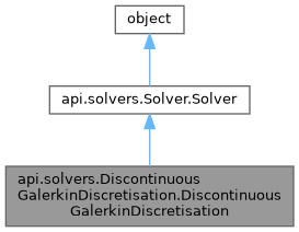
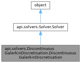
Public Member Functions
	__init__ (self, name, polynomial_degree, dimensions, cell_unknowns, face_unknowns, min_h, max_h, cell_cell_lhs_matrix, cell_cell_rhs_matrix, cell_cell_lhs_matrix_scaling, cell_cell_rhs_matrix_scaling, cell_to_face_matrix, face_to_cell_matrix, cell_to_face_matrix_scaling, face_to_cell_matrix_scaling, face_face_Riemann_problem_matrix, quadrature_points_in_unit_interval, gaussian_integration_points, gaussian_integration_weights)
	Constructor of DG class.
	nodes_per_cell (self)
	nodes_per_face (self)
	add_to_Peano4_datamodel (self, datamodel, verbose)
	Initialise index model.
	add_use_statements (self, observer)
	Register the index numbers to be used in each and every mesh traversal.
	add_to_plot (self, observer)
	Tell the project's observer how to plot the data.
	add_to_create_grid (self, observer)
	Add whatever action set you want to use to observer.
	add_to_enumerate_and_init_solution (self, observer)
	Solution initialisation.
	add_to_assemble (self, observer)
	Add whatever action set you want to use to observer.
	add_to_init_petsc (self, observer)
	Add whatever action set you want to use here.
	add_to_map_solution_onto_mesh (self, observer)
	Add whatever action set you want to use to observer.
	add_implementation_files_to_project (self, namespace, output, subdirectory="")
	The solver creates two classes: An abstract base class and its implementations.
	number_of_matrix_entries_per_vertex (self)
	Nothing is associated with the vertex.
	number_of_matrix_entries_per_face (self)
	In the DG scheme, we have a projection from the left and we have a projection from the right.
	number_of_matrix_entries_per_cell (self)
	This is the actual unknowns per cell.
Public Member Functions inherited from api.solvers.Solver.Solver
	typename (self)
	instance_name (self)
	Return the name of the object that will be created for this solver.
	create_readme_descriptor (self)
	Should really be abstract and properly be initialised.
	name (self)

Data Fields
	polynomial_degree
	dimensions
	cell_unknowns
	face_unknowns
	cell_cell_lhs_matrix
	cell_cell_rhs_matrix
	cell_to_face_matrix
	face_to_cell_matrix
	face_face_Riemann_problem_matrix
	cell_cell_lhs_matrix_scaling
	cell_cell_rhs_matrix_scaling
	cell_to_face_matrix_scaling
	face_to_cell_matrix_scaling
	quadrature_points_in_unit_interval
	gaussian_integration_points
	gaussian_integration_weights
	number_of_matrix_entries_per_cell
	max_h
	min_h
Data Fields inherited from api.solvers.Solver.Solver
	min_h
	max_h

Protected Attributes
	_cell_pde_data
Protected Attributes inherited from api.solvers.Solver.Solver
	_name
	_vertex_petsc_data
	_face_petsc_data
	_cell_petsc_data

Detailed Description

Discontinuous Galerkin Solver with PETSc.

The weak formulation

To translate a PDE into an equation system, we express the solution

\( u = \sum _i u_i \phi _i \)

as sum over shape functions \( \phi _i \). The shape functions in this class are locally continuous, but their linear combination is not. We test this setup against test functions \( v \). Each test function is actually any of the shape functions \( \phi _i \). Drawing both shapes and test functions from the same function space means that we follow a Ritz-Galerkin approach.

Let \( \mathcal{L}(u) \) be the differential operator on the left-hand side of the PDE, i.e. let's assume that we solve

\( \mathcal{L}(u) = f. \)

A weak formulation means that we multiple both sides with a test function and then integrate over the whole thing. As we take all these tests from the same function space as the shape functions, we know that they all have local support.Consequently, our test integral "shrinks" down to the support of the test function

\( \int _\Omega \mathcal{L}(u) \cdot v dx = \int_{\text{cell}_v} \mathcal{L}(u) \cdot v dx \)

as the product disappears everywhere outside of the cell that hosts the test function of interest.

Once again, we can integrate by parts to get rid of the highest derivative in our partial differential operator \( \mathcal{L}(u) \), but this time, we will get an expression of the form

\begin{eqnarray*} \int _\Omega \mathcal{L}(u) \cdot v dx &=& - \int _\Omega \left( \tilde{\mathcal{L}}(u), \nabla v \right) dx + \int _{\partial \text{cell}_v} (n,\tilde{\mathcal{M}}(u)) v dS(x) \\ &=& - \int _{\text{cell}_v} \left( \tilde{\mathcal{L}}(u), \nabla v \right) dx + \int _{\partial \text{cell}_v} (n,\tilde{\mathcal{M}}(\hat u )) v dS(x) \\ & = & \int _{\text{cell}_v} f \cdot v dx. \end{eqnarray*}

We reduced the order of the deriative within \( \mathcal{L}(u) \) and got a new operator \( \tilde{\mathcal{L}} \). If \( \mathcal{L}(u) \) is dominated by a second derivative, \( \tilde{\mathcal{L}} \) hosts only first-order derivatives. But this is a Pyrrhic victory: We now get an additional PDE term over the cell faces.

We conclude that

1. the jump terms along the faces do not disappear, i.e. they do not cancel out from left and right as they do in a Continuous Galerkin formulation.
2. Even worse, they refer to a value \( u \) which technically does not exist, as there is no (unique) solution along the face. We only have a left \( u^- \) and a right \( u^+ \) solution. Therefore, I explicitly write \( \hat u \) in the equation above. It denotes that we haven't yet decided what the function looks like along the face.
3. We now have cell integrals to evaluate, and there are additional face integrals. The latter ones couple neighbouring cells.
   

We end up with a linear equation system

\( A x = b \)

where x has \( |\mathbb{C}| \cdot K \cdot (p+1)^d \) entries. \( \mathbb{C} \) is set of cells in the mesh.

An operator language and temporary variables

Before we dive into examples or discuss how to map this formalism onto code, we introduce an operator language. That is, we break down the overall computation into small tasks. These tasks will be found 1:1 in the code later on. Furthermore, we gain some freedom by breaking things down into tiny bits and pieces: We can alter individual ones or puzzle them together in various ways.

We introduce a few operators (functions) to break down the overall computational scheme into a sequence/set of computations:

• The operator \( A_{cc} \) takes the dofs within a cell and computes the term \( - \int _{\text{cell}_v} \left( \tilde{\mathcal{L}}(u), \nabla v \right) dx \). It takes the \( K (p+1)^d \) values per cell and yields \( K (p+1)^d \) equations/updates from the cell. In classes like petsc.solvers.DiscontinuousGalerkinDiscretisation this matrix is called cell_cell_lhs_matrix.
• Let's introduce temporary variables on the face. Those are the \( u^+ \) and \( u^- \) values, i.e. we store \( 2K (p+1)^{d-1} \) degrees of freedom on the face. Those are not really degrees of freedom. They will be mere projection, i.e. simply encode what the solution along the face is.
• The operator \( A_{cf} \) takes the solution from a cell and projects it onto a face. Let \( u^+ \) and \( u^- \) denote the solution left or right of a face (from the face's point of view). For each of the \( 2d \) faces of a cell, the operator \( P_{cf} \) yields either the \( u^+ \) or \( u^- \).
• The operator \( A_{ff} \) operates on a face. It takes \( u^+ \) and \( u^- \) and yields something that "reconstructs" the solution and applies the flux operator on it. This is the Riemann solver and hence linear algebraises the \( \tilde{\mathcal{M}}(\hat u ) \) from above.
• The operator \( A_{fc} \) takes the \( \hat u \) on the face and yields the updates for the cell. It evaluates \( \int _{\partial \text{cell}_v} (n,\tilde{\mathcal{M}}(\hat u )) v dS(x) \).

Within Peano, it is important to distinguish data on cell and faces carefully from each other. Furthermore (i) we can read data associated with faces within cells; (ii) we can never read data from neighbouring cells within a cell; (iii) we can never access adjacent cell data from a face.

The overall scheme in operator notation thus reads

\( A_{cc} + A_{fc} \circ A_{ff} \circ A_{cf} \)

i.e. we evaluate the cell contributions and add the face contributions which in turn results from a concatenation of three operators: Project solution onto face, solve a Riemann problem there, and then take the result and project it back onto the cell. The projection onto the face is a purely geoemtric thing: Once we know the polynomials chosen within the cell, we can evaluate what the solution looks like depending on the weights (unknowns within the degree of freedom). With that knowledge, we can determine what the solution on the face looks like. We use the same polynomial space there (restricted to the submanifold) and therefore can express the face representation through polynomial weights (left and right of the face), too. For each pair of the polynomial weights, we can solve the Riemann problem and store the outcome in further weights. That is, we represent the outcome of the Riemann problem again in the polynomial space on the faces. Finally, we take this representation, test it against the test functions, integrate over the face and write the contributions back into the cell.

Effectively, our approach blows up the equation system to solve into

\( Ax = \begin{bmatrix} A_{cc} & A_{fc} & 0 & 0 \\ 0 & id & -A_{ff}|_+ & -A_{ff}|_- \\ -id & 0 & A_{cf}|_+ & 0 \\ -id & 0 & 0 & A_{cf}|_- \end{bmatrix} \begin{bmatrix} x_{c} \\ x_f \\ x^+ \\ x^- \end{bmatrix} = \begin{bmatrix} b_{c} \\ 0 \\ 0 \\ 0 \end{bmatrix} \)

where we have to specify the involved matrices further. The \( x_c \) are the real degrees of freedom, i.e. the weights within the cells which effectively span the solution. The \( x_\pm \) encode the projection of these polynomials onto the faces. These are not real degrees of freedom, as they always result directly from the \( x_c \). The \( x_f \) encode the reconstructed solution on the faces and hold the average of the \( x_\pm \) values. This setup means our total matrix is no longer square. \( A_{cc} \) is square, with \( |\mathbb{C}| \cdot (p+1)^d \) rows, where \( |\mathbb{C}| \) is the number of cells in the mesh. \( A_{fc} \) has the same number of rows, but \( |\mathbb{F}| \cdot (p+1)^{d-1} \) columns, since this part has to "hit" \( x_f \). \( A_{ff} \) has \( |\mathbb{F}| \cdot (p+1)^{d-1} \) rows, and twice as many columns (note that \( | x_\pm| \ = \ 2 |x_f| \) ). Finally, \( A_{cf} \) has \( |\mathbb{C}| \cdot (p+1)^d \) rows and \( 2|\mathbb{F}| \cdot (p+1)^{d-1} \) columns, since this part "hits" \( x_\pm \).

Our global matrix is no longer square. We have \( 2 |\mathbb{C}| \cdot (p+1)^d + |\mathbb{F}| \cdot (p+1)^{d-1} \) rows and \( |\mathbb{C}| \cdot (p+1)^d + 3|\mathbb{F}| \cdot (p+1)^{d-1} \) columns.

The write-down as one big matrix as above works if and only if the chosen Riemann solver yield a linear combination of the \( u^-/u^+ \) or \( x^-/x^+ \) values respectively. In many sophisticated solvers, it will not be linear. In this case, the system becomes a non-linear equation system.

Data storage

The data storage within a cell is not prescribed by Peano, i.e. you can, in principle decide if you want to reorder the nodes within the cell or you can decide to order the degrees of freedom overall as SoA as opposed to AoS. At the end of the day, Peano maintains an array of doubles per cell and does not really care about the semantics of those. However, we strongly recommend that you stick to the default configuration where possible:

• Nodes are enumerated following our dimension-generic conventions.
• Data are stored as an Array of Structs (AoS), i.e. first all the unknowns of the first node, then all of the second, and so forth.

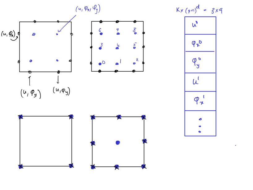
If you change any ordering, you have to take this into account for all associated operators (such as projections onto the faces), but you also will have to amend the plotters which are tied to these conventions.

Data on the faces is

• stored as AoS by default;
• per face, we first store the left projection \( x^- \), then the right projection \( x^+ \) and then the outcome of the flux or associated reconstruction. That is, all the \( x^- \) are held en bloc first before we hold \( x^+ \).
• Per \( x^\pm \), the storage of the nodes and unknowns follows again the dimension-generic conventions.

It is important to recognise that we store three types of quantities per unknown: Its left projection, its right projection, and its outcome which can be either the flux or a reconstructed income. The semantics of the outcome depend upon your operators, i.e. they are not baked into the formalism. Furthermore, there is no assumption about the spacing along the faces. Naturally, you might assume that a Gauss-Lobatto layout within the cell implies a Gauss-Lobatto distribution on the faces. However, no such thing is encoded within the code, as we solely work with operators. They have to encode the correct spacing.

Another assumptions is baked into the realisation as a default: The polynomial degree on the facet result \( x_f \) equals the polynomial degree within the cell.

Examples

Multiple examples are shipped with Peano which demonstrate how to use the plain Discontiuous Galerking solver:

• benchmarks/multigrid/petsc/poisson/dg.py Hosts a simple solver for the Poisson equation. All the rationale are discussed in Poisson equation.

Definition at line 291 of file DiscontinuousGalerkinDiscretisation.py.

Constructor & Destructor Documentation

__init__()

api.solvers.DiscontinuousGalerkinDiscretisation.DiscontinuousGalerkinDiscretisation.__init__	(		self,
			name,
			polynomial_degree,
			dimensions,
			cell_unknowns,
			face_unknowns,
			min_h,
			max_h,
			cell_cell_lhs_matrix,
			cell_cell_rhs_matrix,
			cell_cell_lhs_matrix_scaling,
			cell_cell_rhs_matrix_scaling,
			cell_to_face_matrix,
			face_to_cell_matrix,
			cell_to_face_matrix_scaling,
			face_to_cell_matrix_scaling,
			face_face_Riemann_problem_matrix,
			quadrature_points_in_unit_interval,
			gaussian_integration_points,
			gaussian_integration_weights
	)

Constructor of DG class.

Cell to face projection

Consult Peano's enumeration for multigrid page for info on the ordering. For 2d with a layout as below

the matrix is applied to

\( P_{cf} \begin{bmatrix} x_0^+ \\ x_1^+ \\ x_2^- \\ x_3^- \end{bmatrix} = x_{c} \)

Attributes

Parameters

cell_cell_lhs_matrix	[Float] or [] Pass in [] if you prefer to assemble the matrix per cell yourself. This is the \( \tilde{\mathcal{L}} \) part above. The ordering of the degrees of freedom follows the discussion above. The matrix is from \( K(p+1) \times K(p+1) \).
cell_cell_rhs_matrix	[Float] or [] Pass in [] if you prefer to assemble the matrix per cell yourself. This matrix arises from \( \int f \cdot v \ dx \) and is applied to the nodal values of the PDE within the quadrature nodes of a cell. The matrix is from \( K(p+1) \times K(p+1) \).
cell_cell_lhs_matrix_scaling	Positive integer The lhs matrix is scaled with \( h^x \) where the x is defined by this parameter. If you don't specify an lhs matrix, i.e. you prefer to inject this matrix manually, you can leave this parameter None, as it is not used.
cell_cell_rhs_matrix_scaling	Positive integer The rhs matrix is scaled with \( h^x \) where the x is defined by this parameter. If you don't specify a rhs matrix, i.e. you prefer to inject this matrix manually, you can leave this parameter None, as it is not used.
cell_to_face_matrix	[Float] If you study the global equation system above, you recognise that this matrix is applied to the left or right solutions of a cell's faces.
face_face_Riemann_problem_matrix	[Float] or [] Pass in [] if you prefer to assemble the matrix per cell yourself. This matrix represents the actual Riemann solver. It accepts the left projection \( u^- \) and \( u^+ \) and yields a "reconstructed" value at this point passed into the differential operator. Therefore, this is a band matrix.

Reimplemented from api.solvers.Solver.Solver.

Definition at line 570 of file DiscontinuousGalerkinDiscretisation.py.

References api.solvers.DiscontinuousGalerkinDiscretisation.DiscontinuousGalerkinDiscretisation.__init__().

Referenced by api.solvers.DiscontinuousGalerkinDiscretisation.DiscontinuousGalerkinDiscretisation.__init__().

Here is the call graph for this function:

Here is the caller graph for this function:

Member Function Documentation

add_implementation_files_to_project()

api.solvers.DiscontinuousGalerkinDiscretisation.DiscontinuousGalerkinDiscretisation.add_implementation_files_to_project	(		self,
			namespace,
			output,
			subdirectory = ""
	)

The solver creates two classes: An abstract base class and its implementations.

The abstract base class will be overwritten if there is one in the directory. I pipe all the Python constants into this base class, so they are available in the C++ code.

The implementation file will not be overwritten, as I assume that the users will write their own domain-specific stuff in there. If it does not exist yet, I'll create an empty stub which can be befilled with something meaningful.

Besides the creation of these two files, I also add the files to the project artifacts and the makefile, so they are captured by the build system.

Reimplemented from api.solvers.Solver.Solver.

Definition at line 786 of file DiscontinuousGalerkinDiscretisation.py.

References peano4.api.output.ActionSet.ActionSet.__class__, peano4.api.output.Jinja2TemplatedHeaderImplementationFilePair.Jinja2TemplatedHeaderImplementationFilePair.__class__, and peano4.api.output.TemplatedHeaderFile.TemplatedHeaderFile.__class__.

add_to_assemble()

api.solvers.DiscontinuousGalerkinDiscretisation.DiscontinuousGalerkinDiscretisation.add_to_assemble	(		self,
			observer
	)

Add whatever action set you want to use to observer.

Reimplemented from api.solvers.Solver.Solver.

Definition at line 771 of file DiscontinuousGalerkinDiscretisation.py.

add_to_create_grid()

api.solvers.DiscontinuousGalerkinDiscretisation.DiscontinuousGalerkinDiscretisation.add_to_create_grid	(		self,
			observer
	)

Add whatever action set you want to use to observer.

Reimplemented from api.solvers.Solver.Solver.

Definition at line 747 of file DiscontinuousGalerkinDiscretisation.py.

add_to_enumerate_and_init_solution()

api.solvers.DiscontinuousGalerkinDiscretisation.DiscontinuousGalerkinDiscretisation.add_to_enumerate_and_init_solution	(		self,
			observer
	)

Solution initialisation.

Close to trivial: Just add the action set petsc.actionsets.InitVertexDoFs to the observer.

Reimplemented from api.solvers.Solver.Solver.

Definition at line 751 of file DiscontinuousGalerkinDiscretisation.py.

add_to_init_petsc()

api.solvers.DiscontinuousGalerkinDiscretisation.DiscontinuousGalerkinDiscretisation.add_to_init_petsc	(		self,
			observer
	)

Add whatever action set you want to use here.

I am not sure if there is a real grid traversal tied to this step. So maybe nothing is called. Has to be checked. Anyway, most solvers leave this one blank.

Reimplemented from api.solvers.Solver.Solver.

Definition at line 778 of file DiscontinuousGalerkinDiscretisation.py.

add_to_map_solution_onto_mesh()

api.solvers.DiscontinuousGalerkinDiscretisation.DiscontinuousGalerkinDiscretisation.add_to_map_solution_onto_mesh	(		self,
			observer
	)

Add whatever action set you want to use to observer.

Reimplemented from api.solvers.Solver.Solver.

Definition at line 781 of file DiscontinuousGalerkinDiscretisation.py.

add_to_Peano4_datamodel()

api.solvers.DiscontinuousGalerkinDiscretisation.DiscontinuousGalerkinDiscretisation.add_to_Peano4_datamodel	(		self,
			datamodel,
			verbose
	)

Initialise index model.

There is an index data model, where all the vertices, faces and cells are properly enumerated. This one is taken care of by the superclass. The thing we have to add our our PDE-specific unknowns.

Reimplemented from api.solvers.Solver.Solver.

Definition at line 715 of file DiscontinuousGalerkinDiscretisation.py.

References api.solvers.DiscontinuousGalerkinDiscretisation.DiscontinuousGalerkinDiscretisation._cell_pde_data, and api.solvers.DiscontinuousGalerkinDiscretisation.DiscontinuousGalerkinDiscretisation.add_to_Peano4_datamodel().

Referenced by api.solvers.DiscontinuousGalerkinDiscretisation.DiscontinuousGalerkinDiscretisation.add_to_Peano4_datamodel().

Here is the call graph for this function:

Here is the caller graph for this function:

add_to_plot()

api.solvers.DiscontinuousGalerkinDiscretisation.DiscontinuousGalerkinDiscretisation.add_to_plot	(		self,
			observer
	)

Tell the project's observer how to plot the data.

Nothing fancy here. We add plotters from Peano's toolbox to visualise solution and right-hand side.

Reimplemented from api.solvers.Solver.Solver.

Definition at line 735 of file DiscontinuousGalerkinDiscretisation.py.

add_use_statements()

api.solvers.DiscontinuousGalerkinDiscretisation.DiscontinuousGalerkinDiscretisation.add_use_statements	(		self,
			observer
	)

Register the index numbers to be used in each and every mesh traversal.

You can overwrite the routine and add your own stuff. However, please ensure this routine still is invoked, too.

Reimplemented from api.solvers.Solver.Solver.

Definition at line 730 of file DiscontinuousGalerkinDiscretisation.py.

References api.solvers.DiscontinuousGalerkinDiscretisation.DiscontinuousGalerkinDiscretisation._cell_pde_data, and api.solvers.DiscontinuousGalerkinDiscretisation.DiscontinuousGalerkinDiscretisation.add_use_statements().

Referenced by api.solvers.DiscontinuousGalerkinDiscretisation.DiscontinuousGalerkinDiscretisation.add_use_statements().

Here is the call graph for this function:

Here is the caller graph for this function:

nodes_per_cell()

api.solvers.DiscontinuousGalerkinDiscretisation.DiscontinuousGalerkinDiscretisation.nodes_per_cell

(

self

)

Definition at line 708 of file DiscontinuousGalerkinDiscretisation.py.

References convert::data::PatchData.dimensions, convert::data::Variable.dimensions, mghype.api.matrixgenerators.DLinear.DLinear.dimensions, mghype.api.matrixgenerators.DLinearMassIdentity.DLinearMassIdentity.dimensions, mghype.api.matrixgenerators.GaussLobatto.GaussLobatto.dimensions, mghype.api.matrixgenerators.GaussLobatto.GaussLobattoMatrixFree.dimensions, mghype.api.matrixgenerators.MatrixGenerator.MatrixGenerator.dimensions, api.solvers.DiscontinuousGalerkinDiscretisation.DiscontinuousGalerkinDiscretisation.dimensions, tarch.plotter.api.input.PatchFileParser.UnknownAttributes.dimensions, tarch.plotter.api.input.PatchFileParser.PatchFileParser.dimensions, tarch::reader::PeanoTextPatchFileReader::Header.dimensions, equations.acoustic.Acoustic.dimensions, equations.advection.Advection.dimensions, equations.elastic.Elastic.dimensions, equations.equation.Equation.dimensions, equations.euler.Euler.dimensions, equations.swe.SWE_W_Bathymetry.dimensions, equations.swe.SWE_WO_Bathymetry.dimensions, and api.solvers.DiscontinuousGalerkinDiscretisation.DiscontinuousGalerkinDiscretisation.polynomial_degree.

Referenced by api.solvers.DiscontinuousGalerkinDiscretisation.DiscontinuousGalerkinDiscretisation.number_of_matrix_entries_per_cell().

Here is the caller graph for this function:

nodes_per_face()

api.solvers.DiscontinuousGalerkinDiscretisation.DiscontinuousGalerkinDiscretisation.nodes_per_face

(

self

)

Definition at line 712 of file DiscontinuousGalerkinDiscretisation.py.

References convert::data::PatchData.dimensions, convert::data::Variable.dimensions, mghype.api.matrixgenerators.DLinear.DLinear.dimensions, mghype.api.matrixgenerators.DLinearMassIdentity.DLinearMassIdentity.dimensions, mghype.api.matrixgenerators.GaussLobatto.GaussLobatto.dimensions, mghype.api.matrixgenerators.GaussLobatto.GaussLobattoMatrixFree.dimensions, mghype.api.matrixgenerators.MatrixGenerator.MatrixGenerator.dimensions, api.solvers.DiscontinuousGalerkinDiscretisation.DiscontinuousGalerkinDiscretisation.dimensions, tarch.plotter.api.input.PatchFileParser.UnknownAttributes.dimensions, tarch.plotter.api.input.PatchFileParser.PatchFileParser.dimensions, tarch::reader::PeanoTextPatchFileReader::Header.dimensions, equations.acoustic.Acoustic.dimensions, equations.advection.Advection.dimensions, equations.elastic.Elastic.dimensions, equations.equation.Equation.dimensions, equations.euler.Euler.dimensions, equations.swe.SWE_W_Bathymetry.dimensions, equations.swe.SWE_WO_Bathymetry.dimensions, and api.solvers.DiscontinuousGalerkinDiscretisation.DiscontinuousGalerkinDiscretisation.polynomial_degree.

Referenced by api.solvers.DiscontinuousGalerkinDiscretisation.DiscontinuousGalerkinDiscretisation.number_of_matrix_entries_per_face().

Here is the caller graph for this function:

number_of_matrix_entries_per_cell()

api.solvers.DiscontinuousGalerkinDiscretisation.DiscontinuousGalerkinDiscretisation.number_of_matrix_entries_per_cell

(

self

)

This is the actual unknowns per cell.

Reimplemented from api.solvers.Solver.Solver.

Definition at line 890 of file DiscontinuousGalerkinDiscretisation.py.

References api.solvers.DiscontinuousGalerkinDiscretisation.DiscontinuousGalerkinDiscretisation.cell_unknowns, and api.solvers.DiscontinuousGalerkinDiscretisation.DiscontinuousGalerkinDiscretisation.nodes_per_cell().

Here is the call graph for this function:

number_of_matrix_entries_per_face()

api.solvers.DiscontinuousGalerkinDiscretisation.DiscontinuousGalerkinDiscretisation.number_of_matrix_entries_per_face

(

self

)

In the DG scheme, we have a projection from the left and we have a projection from the right.

These values are proper projections, i.e. they do not carry any semantics. Then we have to solve the Riemann problem, and need one more unknown to store the outcome of that one.

Reimplemented from api.solvers.Solver.Solver.

Definition at line 878 of file DiscontinuousGalerkinDiscretisation.py.

References api.solvers.DiscontinuousGalerkinDiscretisation.DiscontinuousGalerkinDiscretisation.face_unknowns, and api.solvers.DiscontinuousGalerkinDiscretisation.DiscontinuousGalerkinDiscretisation.nodes_per_face().

Here is the call graph for this function:

number_of_matrix_entries_per_vertex()

api.solvers.DiscontinuousGalerkinDiscretisation.DiscontinuousGalerkinDiscretisation.number_of_matrix_entries_per_vertex

(

self

)

Nothing is associated with the vertex.

There's nothing to be done here.

Reimplemented from api.solvers.Solver.Solver.

Definition at line 869 of file DiscontinuousGalerkinDiscretisation.py.

Field Documentation

_cell_pde_data

api.solvers.DiscontinuousGalerkinDiscretisation.DiscontinuousGalerkinDiscretisation._cell_pde_data

protected

Definition at line 688 of file DiscontinuousGalerkinDiscretisation.py.

Referenced by api.solvers.DiscontinuousGalerkinDiscretisation.DiscontinuousGalerkinDiscretisation.add_to_Peano4_datamodel(), and api.solvers.DiscontinuousGalerkinDiscretisation.DiscontinuousGalerkinDiscretisation.add_use_statements().

cell_cell_lhs_matrix

api.solvers.DiscontinuousGalerkinDiscretisation.DiscontinuousGalerkinDiscretisation.cell_cell_lhs_matrix

Definition at line 664 of file DiscontinuousGalerkinDiscretisation.py.

cell_cell_lhs_matrix_scaling

api.solvers.DiscontinuousGalerkinDiscretisation.DiscontinuousGalerkinDiscretisation.cell_cell_lhs_matrix_scaling

Definition at line 670 of file DiscontinuousGalerkinDiscretisation.py.

cell_cell_rhs_matrix

api.solvers.DiscontinuousGalerkinDiscretisation.DiscontinuousGalerkinDiscretisation.cell_cell_rhs_matrix

Definition at line 665 of file DiscontinuousGalerkinDiscretisation.py.

cell_cell_rhs_matrix_scaling

api.solvers.DiscontinuousGalerkinDiscretisation.DiscontinuousGalerkinDiscretisation.cell_cell_rhs_matrix_scaling

Definition at line 671 of file DiscontinuousGalerkinDiscretisation.py.

cell_to_face_matrix

api.solvers.DiscontinuousGalerkinDiscretisation.DiscontinuousGalerkinDiscretisation.cell_to_face_matrix

Definition at line 666 of file DiscontinuousGalerkinDiscretisation.py.

cell_to_face_matrix_scaling

api.solvers.DiscontinuousGalerkinDiscretisation.DiscontinuousGalerkinDiscretisation.cell_to_face_matrix_scaling

Definition at line 672 of file DiscontinuousGalerkinDiscretisation.py.

cell_unknowns

api.solvers.DiscontinuousGalerkinDiscretisation.DiscontinuousGalerkinDiscretisation.cell_unknowns

Definition at line 661 of file DiscontinuousGalerkinDiscretisation.py.

Referenced by api.solvers.DiscontinuousGalerkinDiscretisation.DiscontinuousGalerkinDiscretisation.number_of_matrix_entries_per_cell().

dimensions

api.solvers.DiscontinuousGalerkinDiscretisation.DiscontinuousGalerkinDiscretisation.dimensions

Definition at line 660 of file DiscontinuousGalerkinDiscretisation.py.

Referenced by tarch.plotter.api.input.PatchFileParser.PatchFileParser.__parse_meta_data_region(), tarch.plotter.api.input.PatchFileParser.PatchFileParser.__parse_patch_region(), tarch.plotter.api.input.PatchFileParser.PatchFileParser.__record_doubles_per_patch(), tarch.plotter.api.input.PatchFileParser.UnknownAttributes._initialise_default_mapping_if_no_mapping_specified(), mghype.api.matrixgenerators.MatrixGenerator.MatrixGenerator.convert_index_to_dim(), equations.euler.Euler.eigenvalues(), mghype.api.matrixgenerators.MatrixGenerator.MatrixGenerator.eval_integral(), equations.elastic.Elastic.flux(), equations.euler.Euler.flux(), mghype.api.matrixgenerators.GaussLobatto.GaussLobattoMatrixFree.get_boundary_matrix(), mghype.api.matrixgenerators.GaussLobatto.GaussLobattoMatrixFree.get_cell_from_face_matrix(), mghype.api.matrixgenerators.DLinear.DLinear.get_cell_identity_matrix(), mghype.api.matrixgenerators.DLinearMassIdentity.DLinearMassIdentity.get_cell_identity_matrix(), mghype.api.matrixgenerators.DLinear.DLinear.get_cell_mass_matrix(), mghype.api.matrixgenerators.DLinear.DLinear.get_cell_system_matrix_for_laplacian(), mghype.api.matrixgenerators.DLinearMassIdentity.DLinearMassIdentity.get_cell_system_matrix_for_laplacian(), mghype.api.matrixgenerators.MatrixGenerator.MatrixGenerator.get_deriv(), mghype.api.matrixgenerators.MatrixGenerator.MatrixGenerator.get_points_for_dimension(), mghype.api.matrixgenerators.MatrixGenerator.MatrixGenerator.get_polynomial(), mghype.api.matrixgenerators.GaussLobatto.GaussLobattoMatrixFree.get_projection_matrices(), mghype.api.matrixgenerators.MatrixGenerator.MatrixGenerator.get_weights_for_dimension(), matrices.DgGenerator.getCellToFaceMatrix(), api.solvers.DiscontinuousGalerkinDiscretisation.DiscontinuousGalerkinDiscretisation.nodes_per_cell(), api.solvers.DiscontinuousGalerkinDiscretisation.DiscontinuousGalerkinDiscretisation.nodes_per_face(), and tarch.plotter.api.input.PatchFileParser.PatchFileParser.parse_file().

face_face_Riemann_problem_matrix

api.solvers.DiscontinuousGalerkinDiscretisation.DiscontinuousGalerkinDiscretisation.face_face_Riemann_problem_matrix

Definition at line 668 of file DiscontinuousGalerkinDiscretisation.py.

face_to_cell_matrix

api.solvers.DiscontinuousGalerkinDiscretisation.DiscontinuousGalerkinDiscretisation.face_to_cell_matrix

Definition at line 667 of file DiscontinuousGalerkinDiscretisation.py.

face_to_cell_matrix_scaling

api.solvers.DiscontinuousGalerkinDiscretisation.DiscontinuousGalerkinDiscretisation.face_to_cell_matrix_scaling

Definition at line 673 of file DiscontinuousGalerkinDiscretisation.py.

face_unknowns

api.solvers.DiscontinuousGalerkinDiscretisation.DiscontinuousGalerkinDiscretisation.face_unknowns

Definition at line 662 of file DiscontinuousGalerkinDiscretisation.py.

Referenced by api.solvers.DiscontinuousGalerkinDiscretisation.DiscontinuousGalerkinDiscretisation.number_of_matrix_entries_per_face().

gaussian_integration_points

api.solvers.DiscontinuousGalerkinDiscretisation.DiscontinuousGalerkinDiscretisation.gaussian_integration_points

Definition at line 676 of file DiscontinuousGalerkinDiscretisation.py.

gaussian_integration_weights

api.solvers.DiscontinuousGalerkinDiscretisation.DiscontinuousGalerkinDiscretisation.gaussian_integration_weights

Definition at line 677 of file DiscontinuousGalerkinDiscretisation.py.

max_h

api.solvers.DiscontinuousGalerkinDiscretisation.DiscontinuousGalerkinDiscretisation.max_h

Definition at line 748 of file DiscontinuousGalerkinDiscretisation.py.

Referenced by solvers.api.Solver.Solver.__str__(), exaparty.api.particle.Particle.Particle.readme_descriptor(), and tarch.plotter.api.filters.ExtractMeshResolution.ExtractMeshResolution.render().

min_h

api.solvers.DiscontinuousGalerkinDiscretisation.DiscontinuousGalerkinDiscretisation.min_h

Definition at line 812 of file DiscontinuousGalerkinDiscretisation.py.

Referenced by solvers.api.Solver.Solver.__str__(), exaparty.api.particle.Particle.Particle.readme_descriptor(), and tarch.plotter.api.filters.ExtractMeshResolution.ExtractMeshResolution.render().

number_of_matrix_entries_per_cell

api.solvers.DiscontinuousGalerkinDiscretisation.DiscontinuousGalerkinDiscretisation.number_of_matrix_entries_per_cell

Definition at line 691 of file DiscontinuousGalerkinDiscretisation.py.

polynomial_degree

api.solvers.DiscontinuousGalerkinDiscretisation.DiscontinuousGalerkinDiscretisation.polynomial_degree

Definition at line 659 of file DiscontinuousGalerkinDiscretisation.py.

Referenced by api.solvers.DiscontinuousGalerkinDiscretisation.DiscontinuousGalerkinDiscretisation.nodes_per_cell(), and api.solvers.DiscontinuousGalerkinDiscretisation.DiscontinuousGalerkinDiscretisation.nodes_per_face().

quadrature_points_in_unit_interval

api.solvers.DiscontinuousGalerkinDiscretisation.DiscontinuousGalerkinDiscretisation.quadrature_points_in_unit_interval

Definition at line 675 of file DiscontinuousGalerkinDiscretisation.py.

---

The documentation for this class was generated from the following file:

• src/mghype/petsc/api/solvers/DiscontinuousGalerkinDiscretisation.py