 |
Peano
|
|
Peano
|
This tutorial continues A single black hole with ExaGRyPE: a first (too) trivial setup. There, we evolved a single black hole with first-order Finite Volumes and saw the black hole dissolve: The Rusanov flux adds so much numerical diffusion that the steep profiles around the puncture are smeared out within a few time units. In this tutorial, we switch to the numerical recipe which most numerical relativity codes use, and which we take from GRChombo (https://www.grchombo.org) in particular:
GRChombo furthermore refines the mesh adaptively around the black holes, uses one-sided (lopsided) stencils for the advection terms of the gauge and the moving puncture gauge. We do not mimic these features here, i.e. our setup is similar to GRChombo's, but not the same. We keep the regular mesh, the harmonic slicing and the parameters of the previous tutorial, so we can compare the schemes directly.
We run through the following steps:
As for the previous tutorial, configure Peano with --with-gsl on top of --enable-exagrype, as our initial data stem from TwoPunctures.
The solver is the one of the previous tutorial: a CCZ4 solver with the Gamma driver for the shift and TwoPunctures initial data for a single black hole of mass \( M=1\) at the origin of the domain \( [-9,9]^3\) .
Different to the main run of the previous tutorial, we use Sommerfeld boundary conditions right from the start. They need the solution towards infinity, i.e. the far-field state \( u_\infty\) which the outgoing waves decay to. Far away from the black hole, spacetime is flat: The conformal metric is the identity, the lapse and the conformal factor phi are one, and all other unknowns vanish. The ExaGRyPE library offers exactly this state via exagrype::initialvalues::flat(), so the Sommerfeld term is a one-liner. The origin of the outgoing spherical waves is the puncture, i.e. the default origin of the term.
We wrap the creation into a function, as we will create several projects with different numerical schemes. The Sommerfeld conditions use the maximum eigenvalue of the solver as wave speed. The CCZ4 solver provides it, so there is nothing else to do.
The project follows the final setup of the previous tutorial: \( 9 \times 9 \times 9\) mesh cells with patches of \( 10 \times 10 \times 10\) volumes, i.e. an edge length of \( h=0.2\) , a domain decomposition through SpreadOutOnceGridStagnates, and a plot filter which only writes the patches along the x-axis. Again, we wrap everything into a function which accepts the routine that equips the solver with its numerical scheme:
Our baseline are the Finite Volumes of the previous tutorial, i.e. exahype2.api.fv.RusanovWithExplicitEuler:
With four threads, the run needs 338 time steps of around 1.6 seconds each, i.e. less than ten minutes. The outcome resembles the final runs of the previous tutorial: Next to the puncture, the lapse fills up from 0.26 to 0.86 by \( t=10\) , and the dip along the x-axis flattens out. The Sommerfeld conditions hence do not change the picture, i.e. the reflections at the boundary are not what dissolves our black hole. The Rusanov flux is.
The fourth-order Finite Differences live in exahype2.api.rkfd4. They come with their own numerical scheme, grid construction and plotter, i.e. we replace all three of them:
The data layout hardly changes. Each mesh cell still hosts a patch of \( 10 \times 10 \times 10\) unknowns. We now call them grid cells rather than volumes, as the unknowns are point values in the centres of the grid cells rather than averages over volumes. The puncture hence still sits on a vertex, and the grid cells next to it keep their distance of \( \sqrt{3} h/2 \approx 0.17\) .
What changes is the way we compute the update. Per grid cell, the scheme evaluates the right-hand side of
\begin{eqnarray*} \partial_t Q = - \sum_d B_d(Q) \partial_d Q + S(Q) \end{eqnarray*}
(CCZ4 has no conservative flux), and approximates each derivative through the fourth-order central difference
\begin{eqnarray*} \partial_x Q_i \approx \frac{Q_{i-2} - 8 Q_{i-1} + 8 Q_{i+1} - Q_{i+2}}{12 h}. \end{eqnarray*}
The stencil reaches two grid cells into the neighbouring patches, i.e. each patch is surrounded by a halo of two grid cells. In time, we use the classic fourth-order Runge-Kutta scheme (rk_order=4), i.e. four evaluations of the right-hand side per time step, each with a halo exchange of its own. The time step size follows from the CFL condition with the maximum eigenvalue of CCZ4 as before. Higher-order solvers: Runge Kutta and Finite Differences introduces the scheme for the Euler equations and demonstrates its convergence order.
Everything else carries over: the initial condition, the Sommerfeld conditions, which the scheme applies after each Runge-Kutta stage, the plot filter and the domain decomposition.
We read the lapse along the x-axis with the PointProbe as in the previous tutorial:
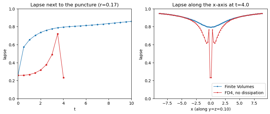
The Finite Differences behave completely differently. For the first time units, they keep the black hole: Next to the puncture, the lapse remains at 0.26 to 0.29 until \( t=1.5\) , where the Finite Volumes have already filled it up to 0.70. Further away from the puncture, the dip is deeper and wider, too. At \( t=4\) , the lapse along the x-axis drops to 0.61 at a distance of around 0.7 from the puncture, whereas the Finite Volumes do not get below 0.79 anywhere.
However, the run does not survive. From \( t \approx 2\) on, the lapse in the grid cells next to the puncture grows (0.32 at \( t=2\) , 0.49 at \( t=3\) , 0.72 at \( t=3.5\) ), and then collapses to 0.23 at \( t=4\) . The profile along the x-axis shows what happens: The two grid cells around the puncture decouple from their neighbours and form a spike, i.e. a sawtooth on the scale of the grid. The conformal factor phi, which has to be positive, becomes negative next to the puncture. Shortly afterwards, the maximum eigenvalue explodes, the time step size collapses to \( 10^{-155}\) at \( t \approx 4.1\) , and the run ends without ever reaching \( t=10\) .
The Finite Differences are also more expensive. Their time step size of around 0.016 is roughly half the one of the Finite Volumes, and each time step evaluates the right-hand side four times. A time step takes around 6.0 seconds rather than 1.6 seconds. Until its collapse after 270 time steps, the run took 27 minutes.
Central differences are neither diffusive nor upwinded. This is what makes them accurate for smooth solutions, but it also means that they cannot remove what they cannot see. Let us study a Fourier mode \( e^{ikx}\) on a grid with spacing \( h\) , which we characterise by \( \theta = kh\) . A mode with small \( \theta\) is smooth, while the mode with \( \theta = \pi\) changes its sign from grid cell to grid cell. The fourth-order central difference turns the derivative \( ik e^{ikx}\) of the mode into \( i \theta_{\text{eff}}/h \cdot e^{ikx}\) with
\begin{eqnarray*} \theta_{\text{eff}} = \frac{8 \sin\theta - \sin 2\theta}{6}. \end{eqnarray*}
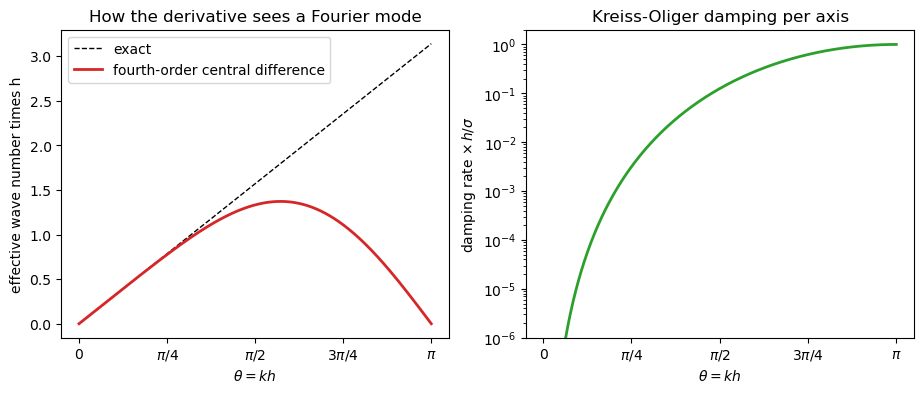
The left picture shows that smooth modes are differentiated correctly, but modes with \( \theta > \pi/2\) are not: Their derivative is underestimated, and the derivative of the mode with \( \theta=\pi\) is zero. The scheme treats this sawtooth like a constant. Any such grid-scale noise hence neither propagates away nor decays. Finite Volumes with a Rusanov flux do not have this problem, as their numerical diffusion damps exactly these modes (and, unfortunately, a lot more).
A black hole is a perfect source of grid-scale noise: Around the puncture, the solution is not smooth, i.e. it is not resolved by any grid, and the CCZ4 equations are nonlinear, i.e. they couple modes. Once grid-scale noise appears, nothing removes it, and it may grow.
Kreiss-Oliger dissipation adds a term to the right-hand side which damps exactly these modes. GRChombo uses the version based upon the sixth derivative, which fits to fourth-order stencils:
\begin{eqnarray*} \partial_t Q = \ldots + \frac{\sigma}{64 h} \sum_d \left( Q_{i-3} - 6 Q_{i-2} + 15 Q_{i-1} - 20 Q_i + 15 Q_{i+1} - 6 Q_{i+2} + Q_{i+3} \right)_d . \end{eqnarray*}
The bracket is \( h^6\) times a discrete sixth derivative, i.e. the term is of order \( \sigma h^5 \partial^6 Q\) . For smooth solutions, it is smaller than the error of our fourth-order stencils, so it does not destroy the convergence order. For the mode \( \theta\) , it yields a damping rate of \( \sigma/h \cdot (4 \sin^2(\theta/2))^3/64\) per axis (right picture): The mode \( \theta=\pi\) is damped with rate \( \sigma/h\) , while smooth modes are hardly touched. The scaling \( \sigma\) is a free parameter. GRChombo's examples typically use a value around \( \sigma = 0.3\) . With explicit time stepping, \( \sigma\) must not be too large, as the dissipation adds the eigenvalue \( -3\sigma/h\) in three dimensions. The fourth-order Runge-Kutta scheme remains stable as long as the time step size times this eigenvalue stays above \( -2.78\) . With our CFL condition, this holds for any reasonable \( \sigma\) .
ExaHyPE's Finite Differences in exahype2.api.rkfd4 deliberately come without any dissipation. ExaGRyPE adds it through a numerical scheme of its own, exagrype.api.FD4WithKODissipation, which is a subclass of exahype2.api.rkfd4.CentralDifferencesWithRungeKutta. Per Runge-Kutta stage, it first evaluates the plain right-hand side, and then runs a second kernel on the same patch which adds the dissipation (exagrype::ccz4::addKreissOligerDissipation()). Both kernels read the same input, i.e. the outcome is the right-hand side with dissipation. As the stencil of the dissipation reaches three grid cells into the neighbours, the scheme widens the halo from two to three grid cells. Everything else is inherited.
To enable the dissipation, we hence only replace the numerical scheme. The grid construction and the plotter remain the ones of exahype2.api.rkfd4:
By default, the dissipation applies to all 59 unknowns. You can restrict it to some of them via their names or indices, e.g. exagrype.api.FD4WithKODissipation( solver, patch_size, rk_order=4, kreiss_oliger_sigma=0.3, quantities=["lapse", "shift", "phi"], ) which damps the lapse, the three components of the shift and phi only.
We run the dissipation with \( \sigma=0.3\) , \( \sigma=1\) and \( \sigma=8\) , which is the value of the legacy ExaGRyPE production runs, and compare against the plain Finite Differences and the Finite Volumes:
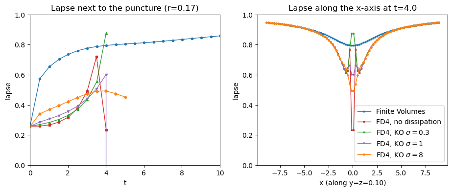
None of the Finite Difference runs reaches \( t=10\) . The dissipation delays the collapse, and the more so the bigger \( \sigma\) is:
| Scheme | Collapse at | Lapse next to the puncture at \( t=1\) | Seconds per time step |
|---|---|---|---|
| Finite Volumes | - (reaches \( t=10\) ) | 0.65 | 1.6 |
| FD4, no dissipation | \( t \approx 4.1\) | 0.27 | 6.0 |
| FD4, KO \( \sigma=0.3\) | \( t \approx 4.3\) | 0.28 | 7.4 |
| FD4, KO \( \sigma=1\) | \( t \approx 4.5\) | 0.31 | 7.0 |
| FD4, KO \( \sigma=8\) | \( t \approx 5.4\) | 0.37 | 6.9 |
With \( \sigma=0.3\) and \( \sigma=1\) , the lapse next to the puncture grows slightly faster than without dissipation during the first time units, but otherwise follows the same pattern: From \( t \approx 2.5\) on, it grows quickly. At \( t=4\) , the profile along the x-axis still shows the spike at the puncture, smaller for \( \sigma=1\) than for \( \sigma=0.3\) . Half a time unit later, the run with \( \sigma=1\) explodes.
With \( \sigma=8\) , the picture changes. Right from the start, the dissipation smooths the dip of the lapse at the puncture a little: Next to the puncture, the lapse is 0.37 at \( t=1\) rather than 0.27, but still far below the 0.65 of the Finite Volumes. It reaches its maximum of 0.49 around \( t=4\) and then decreases again. The profile along the x-axis remains smooth, i.e. there is no spike at the puncture anymore. The dissipation hence removes the grid-scale noise which kills the plain Finite Differences. Nevertheless, the run collapses at \( t \approx 5.4\) : From \( t=4\) on, phi next to the puncture drops (from 0.17 to 0.12 at \( t=5\) ), the time step size shrinks during the final time steps, and then the maximum eigenvalue explodes. Our plots along the x-axis show no sign of this until their last snapshot at \( t=5\) .
The values which GRChombo's examples typically use are hence not sufficient here, and even a very strong dissipation only buys us one more time unit. This is no contradiction to GRChombo: GRChombo combines the dissipation with lopsided stencils for the advection terms of the gauge, the moving puncture gauge with its 1+log slicing, and a much finer mesh around the puncture. With our mesh width of \( h=0.2\) , the horizon spans 2.5 grid cells. These ingredients are the next steps towards a stable long-term evolution with Finite Differences.
The dissipation adds a second kernel per Runge-Kutta stage, which runs over all 59 unknowns. A time step hence takes around 7 rather than 6 seconds, i.e. 16% to 24% longer. The cost does not depend on \( \sigma\) . The differences between the three runs are measurement noise.
To clean up, delete the generated directories. If you rerun the notebook, they are re-created.
The CCZ4 kernels of ExaGRyPE stem from Finite Volume codes. Their non-conservative product, exagrype::ccz4::ncp(), deliberately omits the advection terms \( \beta^k \partial_k Q\) along the shift \( \beta\) for most unknowns, i.e. for K, \( \theta\) , Z, traceK, P and the auxiliary derivatives. As we evolve the shift (CCZ4sk=1), these terms are not zero. All the runs so far hence miss part of the physics.
Codes such as GRChombo add exactly these terms, and they discretise them with lopsided stencils: Fourth-order one-sided differences which are shifted by one grid cell into the direction of the shift,
\( \partial_d Q_i \approx \frac{-3 Q_{i-1} - 10 Q_i + 18 Q_{i+1} - 6 Q_{i+2} + Q_{i+3}}{12 h} \)
for a positive velocity \( \beta_d\) , and mirrored for a negative one. The upwinding damps the grid-scale noise which central differences produce for advection.
Lopsided advection is no CCZ4 specialty. It is hence part of ExaHyPE's Finite Differences: exahype2.api.rkfd4.CentralDifferencesWithRungeKutta accepts the right-hand side kernel CentralDifferencesWithLopsidedAdvection. Per Runge-Kutta stage, this kernel first evaluates the plain right-hand side and then adds \( v_d \partial_d Q_q\) for a velocity v and the advected quantities q (exahype2::fd::addLopsidedAdvection()). The stencil reaches three grid cells into the neighbours, i.e. the scheme uses a halo of three grid cells. ExaGRyPE's CCZ4Solver knows which unknowns its ncp() leaves out and which unknown is the velocity, so we only have to pass these on. FD4WithKODissipation forwards the same arguments, so we can combine lopsided advection with Kreiss-Oliger dissipation:
We run the lopsided advection without dissipation and with Kreiss-Oliger dissipation of \( \sigma=8\) . For the latter, we either damp all 59 unknowns or only Q0-Q22 (G, K, \( \theta\) , Z, the lapse, the shift and b) plus Q53-Q54 (traceK and phi). The second variant leaves the auxiliary first derivatives Q23-Q52 and P undamped:
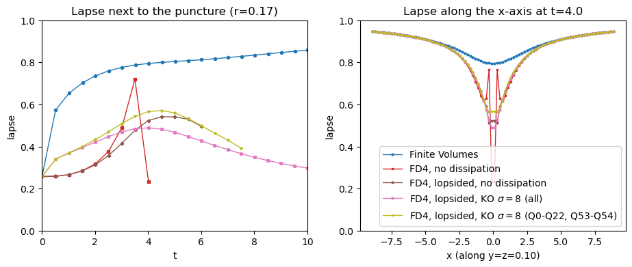
The lopsided advection is the ingredient which we have missed so far:
| Scheme | Collapse at | Lapse next to the puncture at \( t=1\) | Maximum of the lapse next to the puncture |
|---|---|---|---|
| FD4, no dissipation | \( t \approx 4.1\) | 0.27 | - (explodes) |
| FD4, KO \( \sigma=8\) | \( t \approx 5.4\) | 0.37 | 0.49 at \( t \approx 4\) |
| FD4, lopsided, no dissipation | \( t \approx 6.4\) | 0.27 | 0.54 at \( t \approx 5\) |
| FD4, lopsided, KO \( \sigma=8\) (all unknowns) | - (reaches \( t=10\) ) | 0.37 | 0.49 at \( t \approx 4\) |
| FD4, lopsided, KO \( \sigma=8\) (Q0-Q22, Q53-Q54) | \( t \approx 7.6\) | 0.37 | 0.57 at \( t \approx 4.5\) |
Without dissipation, the lopsided advection alone extends the run from \( t \approx 4.1\) to \( t \approx 6.4\) . During the first time units, the lapse next to the puncture is the same as for the plain Finite Differences, as the shift is still small. From \( t \approx 2.5\) on, however, it no longer shoots up, and the profile along the x-axis at \( t=4\) has no spike at the puncture.
Lopsided advection plus Kreiss-Oliger dissipation on all unknowns is the first Finite Difference run which reaches \( t=10\) . Until \( t \approx 4\) , it coincides with the dissipation without lopsided advection. Afterwards, the lapse next to the puncture decreases smoothly to 0.30 at \( t=10\) rather than collapsing. The black hole hence does not dissolve as it does with the Finite Volumes, where the lapse fills up to 0.86.
It matters which unknowns we damp. If we restrict the dissipation to Q0-Q22 and Q53-Q54, the lapse next to the puncture grows faster from \( t \approx 2\) on, and the run collapses at \( t \approx 7.6\) . The auxiliary first derivatives Q23-Q52 and P also develop grid-scale noise, and they need the dissipation, too.
We do not compare the cost per time step here: The machine ran in different power modes during these runs, so their timings are not comparable. A stack sample of a run shows the lopsided kernel in about one in sixty samples, i.e. its cost is small compared to the CCZ4 physics.
 1.9.8