 |
Peano
|
|
Peano
|
In the present application, we solve the underlying problem's Poisson equation by mapping it onto yet another hyperbolic system which evolves on a different time cale.
Our discussion follows the ideas published in
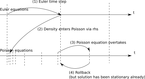
That is, we do not employ an elliptic solver. Instead, we model both equations as hyperbolic equations, where the Euler equations does normal, large time steps. After each time step, the Poisson part of the equation runs many time steps with a tiny time step size until the solution becomes stationary. This is an equivalent to the classic Chorin idea where the Euler step is the prediction, the many tiny Poissonish steps mirror the behaviour of an iterative equation system solver. Its result then enters the overall equation again the right-hand side. We rephrase the latter elliptic equation into a hyperbolic variant with \( \phi (\tau) \) and three helper functions \( (q_1,q_2,q_3)(\tau) \) where
\( \partial _{\tau} \left( \begin{array}{c} \phi \\ q_1 \\ q_2 \\ q_3 \end{array} \right) + \nabla \cdot \left( \begin{array}{ccc} -q_1 & -q_2 & -q_3 \\ -\phi/T_\tau & 0 & 0 \\ 0 & -\phi/T_\tau & 0 \\ 0 & 0 & -\phi/T_\tau \end{array} \right) = \left( \begin{array}{c} -\pi G/\rho \\ -q_1/T_\tau \\ -q_2/T_\tau \\ -q_3/T_\tau \end{array} \right). \)
We will model both equations as completely separate PDEs and hence follow ExaHyPE's generic coupling description. The Poisson
equation \( - \Delta \phi = -\pi G/\rho \) advances on tiny time scales which we indicate by switching from \( Q(t) \) to a \( \phi (\tau) \), i.e. two time arguments \(t\) and \( \tau \). Our strategy is to let the first equation do a large time step, and the second one a tiny one. Then, we take the Euler outcome and feed it into the Poisson equation, which we subsequently advance in time with tiny steps which we increase once the solver runs into a stationary regime. The current \( \rho \) feeds into these tiny time steps as fixed (time-independent) parameter. Once we have reached a stationary state, our Poisson-type solver will use rather huge time steps and eventually overtake the Euler equations. As this poins
The Poisson equation will therefore be restarted at the new time stamp reached by the Euler system.
For the Euler equations, all ingredients are well-known from the introductory example. The Poisson-ish operator is degenerated and yields (for the flux in x-direction)
\( F_x = \left( \begin{array}{c} -q_1 \\ -\phi / T_\tau \\ 0 \\ 0 \end{array} \right) \quad \text{i.e.} \quad \nabla F_x = \left( \begin{array}{cccc} 0 & -1 & 0 & 0 \\ -1/T_\tau & 0 & 0 & 0 \\ 0 & 0 & 0 & 0 \\ 0 & 0 & 0 & 0 \end{array} \right) \)
with a trivial maximum eigenvalue/singular value \( \sqrt{ 1/T_\tau } \). We note that this value does not depend on \( \phi \), i.e. is solution-independent.
In line with ExaHyPE's generic coupling discussion, we go down the route with separate solvers: We simply create two solvers over the corresponding number of unknowns, i.e. 5 for Euler and 4 for the Poisson operator which we have transformed into a stationary first-order hyperbolic system. In applications/exahype2/euler/selfgravitation-with-Poisson/finitevolumes.py, the two solvers are called euler_solver and Poisson_solver.
The interesting thing here is the auxiliary variables: Our Poisson-type equations require the solution's density \( \rho \) of the Euler equation as input. As we want to develop the two solvers completely separate, we introduce a material parameter in the Poisson-type equation which "mirrors" the density of the other equation. For the Poisson implementations, it seems as if the density indeed were some fixed value prescribed by the code. The other way round, our modified Euler requires the gradient from the Poisson equation. In the present example, we hence go down the simplest route and explicitly store the gradient entries as material parameters.
The implementation of the three PDE terms (flux, eigenvalue and source term) is straightforward for both PDEs. Each routine accepts a vector $Q$ which holds both the solution, i.e. five or four components respectively, and then appended to these the one or three "material parameters". For the flux and the eigenvalue, we ignore these material parameters, i.e. the code looks exactly as the plain Euler equations for the first part. The source term applications::exahype2::euler::selfgravitation::Poisson::sourceTerm() however now takes the material parameter as input.
The actual coupling in this example is done by mapping some unknowns from one equation onto material parameters in the other equations. As we deal with a quasi-stationary second PDE, this coupling is trivial in the sense that we do not have to interpolate in time.
The generic coupling discussion clarifies that our code can insert the two-PDE coupling in the data postprocessing or the preprocessing of each time step. In our example here, these two options don't make a difference on the Poisson side, as we will run it until it reaches a stationary state anyway. For the Euler equation, the outcome of the solution has to feed into the subsequent Poisson solutions. Therefore, we run for a coupling after each time step.
For the density, which feeds from the Euler solution into the material parameters of the Poisson-ish equation, we need a plain copy from \( Q[0]|_{\text{Euler}} \mapsto Q[4]|_{\text{Poisson}} \) for which ExaHyPE's toolbox provides the generic implementation toolbox::blockstructured::copyUnknown(). We can insert it straight into the postprocessing on the Python API level:
In this special case, we use a plain copy. If the two different solvers have different patch sizes, i.e. unknowns per dimension, we have to interpolate accordingly. The invocation is kind of self-explaining: We include a helper function from the toolbox and call the copyUnknown. The "nasty" part is the fineGridCellPoissonQ part, for which we have to study the naming conventions within —a detail usually hidden from the user: The unknowns per cell (so the plain double array) are called fineGridCell followed by the name of the solver Euler and then a Q. The data is actually a struct for our plain double fields which hosts a pointer value.
If you work in the preprocessing step, i.e. inject the coupling prior to the time step, you work with a temporary array reconstructedPatch which hosts the patch data plus the information from the halos. That is, you work with some fineGridCell...Q value as pre-image, but you write into reconstructedPatch which now already has a halo. You can also hook into this step to "save" data from reconstructedPatch before it is handed over to the time stepping.
For the coupling the other way round, we follow exactly the same principle. There is room for optimisation here, as we would only have to couple after the Poisson equation has run into a stationary solution, but I omit such optimisations here. I simple invoke the mapping
\( Q[0] _{\text{Poisson}} = \phi \mapsto \left( \begin{array}{c} \partial _x \phi \\ \partial _y \phi \\ \partial _z \phi \end{array} \right) = \left( \begin{array}{c} Q[5] \\ Q[6] \\ Q[7] \end{array} \right)_{\text{Euler}} \)
after each and every solver update step. Again, ExaHyPE offers a premanufactured mapping for this already, so we simply invoke toolbox::blockstructured::computeGradientAndReturnMaxDifference():
So far, we couple the two solvers in each and every time step. This makes no sense, if the two solvers don't run in-sync, i.e. with exactly the time step size. For the coupling in time, we exploit some simple properties of any ExaHyPE solver:
GlobalAdaptiveTimeStep or literally any solver that does not use fixed time step sizes, we can tweak the time step sizes to meet our needs.Therefore, we first switch to an adaptive time stepping scheme. The Poisson solver usually employs a smaller relaxation of the time step size. Our strategy for a coupled solver is to add one more boolean evaluation to the time step guard of these adaptive solvers. As we have two solvers per cell (Poisson and Euler), the cell hosts two time stamps and the guard can compare these two time stamps. In our example, we know that the Poisson solver always is the slow solver. In a first step, we thus have to throttle down the Euler solver. It has to wait for its cousin solver:
Throughout the coupling example, I take two existing solvers and modify/augment their attributes. In a larger code, it might be reasonable to create two completely new Python classes which inherit from the respective solvers, i.e. to model them as real new solvers. A lot of the string construction above violates object-oriented information hiding paradigms, so it might be better to accommodate it within classes of their own.
Next, we have to make a decision how to handle the paper's original idea that the Poisson solver should run into a stationary solution before we actually progress in time. In a world with a fixed global time step, this can be achieved by making the time step of the Poisson solver extremely small. We then get hundreds and thousands of Poisson time steps per Euler step and "just" have to ensure that these Poisson steps are sufficient to obtain an almost stationary solution just before Euler hops in time once again. This approach quickly becomes computationally infeasible. We need an approach that switches gears once we are stationary.
By default, the Poisson solver will not use huge time steps once it approaches a stationary solution. Alternatively, it might take a huge one (should the eigenvalues approach 0) and yield some outputs which make no sense, i.e. host timestamps which are way beyond the terminal simulation time. We are well-advised to introduce some more modest time stepping.
To determine if the solver is (close to) stationary, we evaluate the difference between the gradient of \( \phi \) after each Poisson step. For this, we tweak the coupling term:
The new computation preserves the semantics of the old one plus computes a value delta which it then pipes into the Poisson solver object. Here, we once again exploit our knowledge about 's internal working and naming conventions. To make the whole thing finally work, we tweak the Poisson solver:
delta as we have computed it above. 1.9.8