Peano
Loading...
Searching...
No Matches
solvers.api.DiscontinuousGalerkinDiscretisationPointWiseRiemannSolver.DiscontinuousGalerkinDiscretisationPointWiseRiemannSolver Class Reference

Most efficient solver we have for this type of problem class. More...

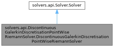
Inheritance diagram for solvers.api.DiscontinuousGalerkinDiscretisationPointWiseRiemannSolver.DiscontinuousGalerkinDiscretisationPointWiseRiemannSolver:
Collaboration diagram for solvers.api.DiscontinuousGalerkinDiscretisationPointWiseRiemannSolver.DiscontinuousGalerkinDiscretisationPointWiseRiemannSolver:

Public Member Functions

 __init__ (self, name, dimensions, poly_degree, unknowns_per_cell_node, solutions_per_face_node, projections_per_face_node, min_h, max_h, assembly_matrix, assembly_matrix_scaling, mass_matrix, mass_matrix_scaling, face_from_cell_projection, face_from_cell_projection_scaling, cell_from_face_projection, cell_from_face_projection_scaling, riemann_matrix, boundary_matrix, cell_relaxation, face_relaxation, approximate_system_matrix, approximate_system_matrix_scaling, integration_points, solver_tolerance, custom_init_actionset=None, custom_plot_actionset=None, custom_init_cell="", enable_plotting=True, plot_predicate="true", solver_includes="", use_smart_pointer=True, track_solution_between_cycles=False)
 Construct the solver.
 
- Public Member Functions inherited from solvers.api.Solver.Solver
 add_to_Peano4_datamodel (self, datamodel, verbose)
 
 add_use_statements (self, observer)
 This routine should still be called even if overwritten in child class.
 
 typename (self)
 
 instance_name (self)
 Return the name of the object that will be created for this solver.
 
 create_readme_descriptor (self)
 
 add_to_abstract_solver (self, header, implementation)
 
 add_to_vertex_data (self, name, size)
 Add in extra attributes on the fly.
 
 add_to_cell_data (self, name, size)
 Add in extra attributes on the fly.
 
 add_to_face_data (self, name, size)
 Add in extra attributes on the fly.
 
 name (self)
 
 __str__ (self)
 

Protected Attributes

 _dimensions
 
 _poly_degree
 
 _unknowns_per_cell_node
 
 _solutions_per_face_node
 
 _projections_per_face_node
 
 _assembly_matrix
 
 _assembly_matrix_scaling
 
 _mass_matrix
 
 _mass_matrix_scaling
 
 _face_from_cell_projection
 
 _face_from_cell_projection_scaling
 
 _cell_from_face_projection
 
 _cell_from_face_projection_scaling
 
 _riemann_matrix
 
 _boundary_matrix
 
 _approximate_system_matrix
 
 _approximate_system_matrix_scaling
 
 _cell_relaxation
 
 _face_relaxation
 
 _solver_tolerance
 
 _solver_includes
 
 _custom_init_actionset
 
 _custom_plot_actionset
 
 _custom_init_cell
 
 _enable_plotting
 
 _plot_predicate
 
 _integration_points
 
 _track_solution_between_cycles
 
 _unknowns_per_cell
 
 _unknowns_per_face_solution
 
 _unknowns_per_face_projection
 
 _use_smart_pointer
 
- Protected Attributes inherited from solvers.api.Solver.Solver
 _name
 
 _vertex_data
 
 _face_data
 
 _cell_data
 
 _abstract_solver_header_extras
 
 _abstract_solver_implementation_extras
 

Additional Inherited Members

- Data Fields inherited from solvers.api.Solver.Solver
 min_h
 
 max_h
 

Detailed Description

Most efficient solver we have for this type of problem class.

You can find each of the action sets here: solvers.api.actionsets.DGSolver.InitHigherOrderDofs.InitHigherOrderDofs

The text below specifies the semantics and behaviour of this matrix-free DG solver. A tutorial running step by step through the steps how to use it can be found in the tutorials section. The solver in general tackles a PDE

\( \mathcal{L}(u) = f \)

resulting in a linear equation system

\( Au = b. \)

Throughout the discussion, we unfold the compute steps over the compute mesh.

Storage

This solver holds \( K^c (p+1)^d \) unknowns (doubles) per cell for the solution, \( K^c (p+1)^d \) per cell for the right-hand side, and the same number for the residual. Holding the residual in the cell allows us to separate some algorithm steps into different action sets. In particular, we project the face solution back into the cells after updating the cell solution (in separate sweeps). These are the primary variables, i.e. those directly resulting from the PDE formulation. The correspond to the unknowns directly from \( u \) and the right-hand side.

Further to that, we hold auxiliary variables on the faces: Our Riemann solver accepts the left and the right solution. Here, each degree of freedom has \( K^f_{f \gets c} \) unknowns. It will return a result (the flux), which has \( K^f \) unknowns. Per face node, we hence hold, in total, \( ( K^f + 2K^f_{f \gets c} ) (p+1)^{d-1} \) unknowns. That is the solution for each unknown per face node, as well as a projection from the left and right for each unknown per cell. \( K^c \) and \( K^f \) can be different, but often they are the same. The user can choose how many of the \( K^c \) to project onto the face by modifying \( K^f_{f \gets c} \).

Operators

With the auxiliary variables, in place, we can write down the DG problem as

\( \left( \begin{array}{cccc} A^{cc} & & & P_{c \gets f} \\ P_{f \gets c} & id & & \\ P_{f \gets c} & & id \\ & id & id & A^{ff} \end{array} \right) \left( \begin{array}{c} u^c \\ u^+ \\ u^- \\ q \end{array} \right) = \left( \begin{array}{c} M b \\ 0 \\ 0 \\ 0 \end{array} \right) \)

in line with xxxx. The \( q \) is the result of the Riemann solver.

Solver

We now realise a Block-Jacobi smoother subject to two relaxation parameters \( \omega _c, \omega _f \in [0,1] \). We tackle the first line in the block system with one smoothing step of a stationary iterative scheme, solve two and three exact (as they are trivial with the identity on the diagonal) and apply Jacobi to the last row again. As the first and last block are updated in parallel by the Jacobi scheme, the resuling algorithm is globally a Jacobi relaxation, too.

  • Per cell, we tackle the equation \( A^{cc} u^c + P_{c \gets f} q = M b \) which yields the update rule

    \begin{eqnarray*} u|_c & \gets & u|_c + \omega _c \tilde {A}^{-1}\left( Mb - A^{cc} u^c - P_{c \gets f} q \right). \end{eqnarray*}

    Here, the \( q \) is the solution of the PDE term on the faces which we assume to be fixed. At this point, we are quite generic and dump the responsibility onto the user to give us an approximation of \( A_{cc} \) that we can invert. Notably, we highlight that the user may give us \( \tilde{A} = A^{cc} \) in a DG sense, as we cannot invert \( A^{cc} \).
  • Per face, we use a plain Jacobi. We assume that we have an explicit expression of the Riemann solution (simple averaging would be an example) and hence \( \hat A = id \). We consequently get

    \begin{eqnarray*} q|_f & \gets & q|_f + \omega _f \left( \mathcal{R}(u^-, u^+) - q|_f \right) \\ & = & (1-\omega _f) q|_f + \omega _f \mathcal{R}(u^-, u^+). \end{eqnarray*}

Algorithmical blueprint

  1. Enter cell: Whenever a cell is entered, we create a temporary \( K^c(p+1)^d \) array (on the heap).
    1. Into this temporary array \( r \), we write \( Mb \). This is the mass matrix (right-hand side matrix of the class constructor, as we are not restricted to a traditional mass matrix) times the right-hand sides within the cell. So \( r \gets Mb. \)
    2. Once complete, we substract \( P^{c \gets f} q|_f \). That is, we take the solution on the face and we project it (cell from face) onto the cell, where we substract it from the previous \( r \) value. We also do the same with the cell-to-cell couplings. So: \( r \gets Mb - Pq|_f -A^{cc}u^c. \) We also do the same with the cell couplings
    3. The third step is where the MFlops come from: We take the user's approximation of the cell matrix and explicitly invert it. For a linear, invariant matrix \( A \), we could do so once, but the solver itself makes no assumption if the matrix is invariant or not. So it inverts it every step and uses BLAS routines or this. The result is multiplied with the residual as accumulated so far: \( r \gets \tilde{A}^{-1} \left( Mb - Pq|_f -A^{cc}u^c \right). \)
    4. We run over the solution within the cell and scale each entry with \( (1-\omega _c) \). If \( \omega _c =1 \), this means we set the entries to zero. In general, the entries however will only be damped. After that, we add the \( r \) values to each point. This gives us a new solution guess.
    5. We project the updated solution \( u|_c \) onto the faces, i.e. obtain a new \( u|_f^{\pm } \). This is realised within the action set ProjectOntoFaces.
  2. touchFaceFirstTime(): Whenever a face is touched, we solve the Riemann problem and update the Riemann guess accordingly. Initially, we assume that the \( q \) entries on the face are all set to zero.

    1. We evaluate per node on the face the expression \( \mathcal{R}(u^-,u^+) \). For this, we loop over the \( (p+1)^{d-1} \) points and call the C++ solver's routine. The user can thus implement the actual Riemann solver themself.
    2. We take the result and update the value on the face according to \( q|_f \gets (1-\omega _f) q|_f + \omega _f \mathcal{R}(u^-, u^+). \)

    All of this functionality can be found in the subpackage actionsets.UpdateResidual.

How does it work?

Python stuff

There is a very simple Poisson solver tutorial in the tutorials section which illustrates how to use this solver.

The user needs to supply a few crucial matrices, referred to in the maths above. These are noted and their shapes discussed in the parameters section of the documentation of this class.

Under the hood

Inside the cells we store \( K^c (p+1)^{d} \) values for the solution, and the same number for the rhs and residual. We store the residual in the cell so that we can calculate the update to the cell solution separately from the projection of face solution back into the cells, but crucially are able to update the global residual before we apply the preconditioner. On each face we store \( K^f (p+1)^{d-1} \) values for the solution, and then \( 2K^f_{f \gets c} (p+1)^{d-1} \) for the projections in a separate array. We note that this factor of two comes from the fact that we have projections from cells on both the left and right. The user is free to choose how many variables from the cell they want to project onto the face. The value K^f_{f \gets c} is exposed in dg.py as the argument --projections_per_face"</tt>. @subsubsection autotoc_md211 Matrices we pass in to the solver class See documentation for this class itself... So far we have three non-trivial action sets. @subsubsection autotoc_md212 InitHigherOrderDofs Code for this is in actionsets.InitHigherOrderDofs. So far nothing happens, other than determining which cells/faces are on the boundary and putting in initial guesses for each cell and face dof. We pass over to the implementation cpp file which should be left in situ in the directory for the application. @subsubsection autotoc_md213 UpdateFaceSolution Code for this is in actionsets.DGSolver.UpdateFaceSolution. This action set only contains something nontrivial at touchFaceFirstTime. We apply the Riemann matrix that is present in the Abstract Solver class. This action set goes first, the idea being that we updated the face solution using the updated face projections from the previous sweep. @subsubsection autotoc_md214 ProjectIntoCellAndUpdateCellSolution Code for this is in actionsets.DGSolver.ProjectIntoCellAndUpdateCellSolution. This action set works when we touch the cell for the first time. We project the newly updated face solution back into the cells. In particular we: - Write the updated face solution into the residual stored in the cell. This finishes the cell update from the previous sweep. - Update the global residual - Update the cell solution, which is projected back onto faces in the next action set. @subsubsection autotoc_md215 ProjectOntoFaces Code for this is in actionsets.DGSolver.ProjectOntoFaces. This occurs strictly after ProjectIntoCellAndUpdateCellSolution, so that we project freshly updated Cell values onto the Faces. @subsubsection autotoc_md216 UpdateResidual Code for this is in actionsets.DGSolver.UpdateResidual. We do something nontrivial in touchCellFirstTime, namely perform the cell update rule as above. We set the residual to be \_form#322. @param solver_includes C++ code snippet Arbitrary C++ code snippet. Usually used to include additional files (therefore the name), though you can use it for preprocessing macros or using statements as well. Has to be a valid C++ expression, i.e. something similar to @icode #include "myfile.h"

Definition at line 21 of file DiscontinuousGalerkinDiscretisationPointWiseRiemannSolver.py.

Constructor & Destructor Documentation

◆ __init__()

solvers.api.DiscontinuousGalerkinDiscretisationPointWiseRiemannSolver.DiscontinuousGalerkinDiscretisationPointWiseRiemannSolver.__init__ (   self,
  name,
  dimensions,
  poly_degree,
  unknowns_per_cell_node,
  solutions_per_face_node,
  projections_per_face_node,
  min_h,
  max_h,
  assembly_matrix,
  assembly_matrix_scaling,
  mass_matrix,
  mass_matrix_scaling,
  face_from_cell_projection,
  face_from_cell_projection_scaling,
  cell_from_face_projection,
  cell_from_face_projection_scaling,
  riemann_matrix,
  boundary_matrix,
  cell_relaxation,
  face_relaxation,
  approximate_system_matrix,
  approximate_system_matrix_scaling,
  integration_points,
  solver_tolerance,
  custom_init_actionset = None,
  custom_plot_actionset = None,
  custom_init_cell = "",
  enable_plotting = True,
  plot_predicate = "true",
  solver_includes = "",
  use_smart_pointer = True,
  track_solution_between_cycles = False 
)

Construct the solver.

Please consult the tutorial on data masking for a discussion of the load_store_compute_flag settings.

Parameters
poly_degreeInteger The degree of the polynomial that we use. Has to be bigger or equal to one.
unknowns_per_cell_nodePositive Integer This is the \( K^c \) from the solver description.
solutions_per_face_nodePositive Integer This is the \( K^f \) from the solver description.
projections_per_face_nodePositive Integer This is the \( K^f_{f \gets c} \) from the solver description.
cell_relaxationFloat
This is the \( \omega _c \) from the description above and typically chosen form \( ]0,1[ \) though some scenarios benefit from a slight overrelaxation.
assembly_matrix\( \mathbb{R}^{K^c * (p+1)^{d} \times K^c * (p+1)^{d}}\) This is the cell-to-cell matrix which defines how the cell nodes couple to one another. Is is a square matrix. You can pass in None. In this case, the generated C++ code will not compile, but you will be allowed to fill it in manually.
assembly_matrix_scaling\( \mathbb{R}^{K^c * (p+1)^{d} \times K^c * (p+1)^{d}}\) This is a matrix of ints that prescribes how we scale each element in the assembly_matrix ie for each i,j, we do: assembly_matrix[i,j] *= ( h )^( assembly_matrix_scaling[i,j] )
mass_matrix\( \mathbb{R}^{K^c * (p+1)^{d} \times K^c * (p+1)^{d}}\)
mass_matrix_scaling\( \mathbb{R}^{K^c * (p+1)^{d} \times K^c * (p+1)^{d}}\) This is a matrix of ints that prescribes how we scale each element in the mass_matrix ie for each i,j, we do: mass_matrix[i,j] *= ( h )^( mass_matrix_scaling[i,j] )
face_from_cell\( \mathbb{R}^{2d * 2K^f_{f \gets c} * (p+1)^{d-1} \times K^c * (p+1)^{d}}\) This matrix projects the cell solution onto all of the faces. Note the extra factor of \( 2d \). The structure of this matrix is quite important. The rows should be structured in blocks of \( 2K^f_{f \gets c} * (p+1)^{d-1} \), ie one for each face, in the familiar Peano ordering. We note that this is the same as the number of projections we store per face. We note that, since the 0th face has left-side projections which should be set outside of the cell, that at least half of the rows of the matrix should be empty. We also note that each face contains multiple nodes, and they should be ordered sequentially in the typical Peano fashion, i.e. greedily along each coordinate axis until full, starting from the negative. For each face, with two nodes, with two values (q and u) being projected onto the face, the rows should be ordered as follows:
  1. Negative projection of q onto node 0
  2. Negative projection of q onto node 1
  3. Negative projection of u onto node 0
  4. Negative projection of u onto node 1
  5. Positive projection of q onto node 0
  6. Positive projection of q onto node 1
  7. Positive projection of u onto node 0
  8. Positive projection of u onto node 1 In two dimensions, all of the negative projections should be 0 on faces 0 and 1. Ditto for the positive projections on faces 2 and 3.
cell_from_face\( \mathbb{R}^{K^c * (p+1)^{d} \times 2d K^f * (p+1)^{d-1}}\) This matrix projects the face solution onto the cells. Note the extra factor of \( 2d \), similar to face_from_cell matrix. Some clever indexing is required in the backend here. The enumeration of the cols should follow a similar pattern to the rows of face_from_cell.
cell_from_face_scaling\( \mathbb{R}^{K^c * (p+1)^{d} \times 2d K^f * (p+1)^{d-1}}\) This is a matrix of ints that prescribes how we scale each element in the cell_from_face ie for each i,j, we do: cell_from_face[i,j] *= ( h )^( cell_from_face_scaling[i,j] )
Riemann_matrix\( \mathbb{R}^{ K^f (p+1)^{d-1} \times 2K^f_{f \gets c} (p+1)^{d-1}} \) The matrix that combines the left/right projections on the cell and outputs a value which determines \( q \).
face_relaxationFloat This is the \( \omega _f \) from above. Chosen from \( ]0,1[ \).
approximate_system_matrix\( \mathbb{R}^{K^c (p+1)^d \times K^c (p+1)^d} \) Approximation \( \tilde{A} \) which will be internally inverted, so it has to be non-singular.
approximate_system_matrix_scaling\( \mathbb{R}^{K^c (p+1)^d \times K^c (p+1)^d} \)
integration_points[Float] Sequence of polynomial_degree+1 entries which identify the position of the integration points along the unit interval.

Reimplemented from solvers.api.Solver.Solver.

Reimplemented in solvers.api.DiscontinuousGalerkinDiscretisationPointWiseRiemannSolver_Tasks.DiscontinuousGalerkinDiscretisationPointWiseRiemannSolver_Tasks, and solvers.api.DiscontinuousGalerkinDiscretisationPointWiseRiemannSolver_Unshifted.DiscontinuousGalerkinDiscretisationPointWiseRiemannSolver_Unshifted.

Definition at line 252 of file DiscontinuousGalerkinDiscretisationPointWiseRiemannSolver.py.

References solvers.api.DiscontinuousGalerkinDiscretisationPointWiseRiemannSolver.DiscontinuousGalerkinDiscretisationPointWiseRiemannSolver.__init__().

Referenced by solvers.api.DiscontinuousGalerkinDiscretisationPointWiseRiemannSolver.DiscontinuousGalerkinDiscretisationPointWiseRiemannSolver.__init__().

Here is the call graph for this function:
Here is the caller graph for this function:

Field Documentation

◆ _approximate_system_matrix

solvers.api.DiscontinuousGalerkinDiscretisationPointWiseRiemannSolver.DiscontinuousGalerkinDiscretisationPointWiseRiemannSolver._approximate_system_matrix
protected

◆ _approximate_system_matrix_scaling

solvers.api.DiscontinuousGalerkinDiscretisationPointWiseRiemannSolver.DiscontinuousGalerkinDiscretisationPointWiseRiemannSolver._approximate_system_matrix_scaling
protected

◆ _assembly_matrix

solvers.api.DiscontinuousGalerkinDiscretisationPointWiseRiemannSolver.DiscontinuousGalerkinDiscretisationPointWiseRiemannSolver._assembly_matrix
protected

◆ _assembly_matrix_scaling

solvers.api.DiscontinuousGalerkinDiscretisationPointWiseRiemannSolver.DiscontinuousGalerkinDiscretisationPointWiseRiemannSolver._assembly_matrix_scaling
protected

◆ _boundary_matrix

solvers.api.DiscontinuousGalerkinDiscretisationPointWiseRiemannSolver.DiscontinuousGalerkinDiscretisationPointWiseRiemannSolver._boundary_matrix
protected

◆ _cell_from_face_projection

solvers.api.DiscontinuousGalerkinDiscretisationPointWiseRiemannSolver.DiscontinuousGalerkinDiscretisationPointWiseRiemannSolver._cell_from_face_projection
protected

◆ _cell_from_face_projection_scaling

solvers.api.DiscontinuousGalerkinDiscretisationPointWiseRiemannSolver.DiscontinuousGalerkinDiscretisationPointWiseRiemannSolver._cell_from_face_projection_scaling
protected

◆ _cell_relaxation

solvers.api.DiscontinuousGalerkinDiscretisationPointWiseRiemannSolver.DiscontinuousGalerkinDiscretisationPointWiseRiemannSolver._cell_relaxation
protected

◆ _custom_init_actionset

◆ _custom_init_cell

solvers.api.DiscontinuousGalerkinDiscretisationPointWiseRiemannSolver.DiscontinuousGalerkinDiscretisationPointWiseRiemannSolver._custom_init_cell
protected

◆ _custom_plot_actionset

◆ _dimensions

◆ _enable_plotting

◆ _face_from_cell_projection

solvers.api.DiscontinuousGalerkinDiscretisationPointWiseRiemannSolver.DiscontinuousGalerkinDiscretisationPointWiseRiemannSolver._face_from_cell_projection
protected

◆ _face_from_cell_projection_scaling

solvers.api.DiscontinuousGalerkinDiscretisationPointWiseRiemannSolver.DiscontinuousGalerkinDiscretisationPointWiseRiemannSolver._face_from_cell_projection_scaling
protected

◆ _face_relaxation

solvers.api.DiscontinuousGalerkinDiscretisationPointWiseRiemannSolver.DiscontinuousGalerkinDiscretisationPointWiseRiemannSolver._face_relaxation
protected

◆ _integration_points

solvers.api.DiscontinuousGalerkinDiscretisationPointWiseRiemannSolver.DiscontinuousGalerkinDiscretisationPointWiseRiemannSolver._integration_points
protected

◆ _mass_matrix

solvers.api.DiscontinuousGalerkinDiscretisationPointWiseRiemannSolver.DiscontinuousGalerkinDiscretisationPointWiseRiemannSolver._mass_matrix
protected

◆ _mass_matrix_scaling

solvers.api.DiscontinuousGalerkinDiscretisationPointWiseRiemannSolver.DiscontinuousGalerkinDiscretisationPointWiseRiemannSolver._mass_matrix_scaling
protected

◆ _plot_predicate

◆ _poly_degree

solvers.api.DiscontinuousGalerkinDiscretisationPointWiseRiemannSolver.DiscontinuousGalerkinDiscretisationPointWiseRiemannSolver._poly_degree
protected

◆ _projections_per_face_node

solvers.api.DiscontinuousGalerkinDiscretisationPointWiseRiemannSolver.DiscontinuousGalerkinDiscretisationPointWiseRiemannSolver._projections_per_face_node
protected

◆ _riemann_matrix

solvers.api.DiscontinuousGalerkinDiscretisationPointWiseRiemannSolver.DiscontinuousGalerkinDiscretisationPointWiseRiemannSolver._riemann_matrix
protected

◆ _solutions_per_face_node

◆ _solver_includes

solvers.api.DiscontinuousGalerkinDiscretisationPointWiseRiemannSolver.DiscontinuousGalerkinDiscretisationPointWiseRiemannSolver._solver_includes
protected

◆ _solver_tolerance

solvers.api.DiscontinuousGalerkinDiscretisationPointWiseRiemannSolver.DiscontinuousGalerkinDiscretisationPointWiseRiemannSolver._solver_tolerance
protected

◆ _track_solution_between_cycles

solvers.api.DiscontinuousGalerkinDiscretisationPointWiseRiemannSolver.DiscontinuousGalerkinDiscretisationPointWiseRiemannSolver._track_solution_between_cycles
protected

◆ _unknowns_per_cell

solvers.api.DiscontinuousGalerkinDiscretisationPointWiseRiemannSolver.DiscontinuousGalerkinDiscretisationPointWiseRiemannSolver._unknowns_per_cell
protected

◆ _unknowns_per_cell_node

solvers.api.DiscontinuousGalerkinDiscretisationPointWiseRiemannSolver.DiscontinuousGalerkinDiscretisationPointWiseRiemannSolver._unknowns_per_cell_node
protected

◆ _unknowns_per_face_projection

solvers.api.DiscontinuousGalerkinDiscretisationPointWiseRiemannSolver.DiscontinuousGalerkinDiscretisationPointWiseRiemannSolver._unknowns_per_face_projection
protected

◆ _unknowns_per_face_solution

solvers.api.DiscontinuousGalerkinDiscretisationPointWiseRiemannSolver.DiscontinuousGalerkinDiscretisationPointWiseRiemannSolver._unknowns_per_face_solution
protected

◆ _use_smart_pointer

solvers.api.DiscontinuousGalerkinDiscretisationPointWiseRiemannSolver.DiscontinuousGalerkinDiscretisationPointWiseRiemannSolver._use_smart_pointer
protected

The documentation for this class was generated from the following file: