Prepare the show

import sys, os
 
sys.path.insert(0, os.path.abspath("../../../python/"))
 
import peano4.api, exahype2

This time, we employ a different numerical scheme: ADER-DG. From a user's perspective, ADER-DG has a slightly different signature compare to Finite Volumes: Besides the name, the unknowns, and so forth, it needs a polynomial order, and it speaks of cell sizes for the mesh and not finite volume sizes. At this point, this is the only difference to the schemes employed before.

unknowns = {"h": 1, "hu": 2, "b": 1}
auxiliary_variables = {}
max_h = 1.1 * 2.0 / (3.0 ** 3)
min_h = max_h
 
my_solver = exahype2.solvers.aderdg.GlobalAdaptiveTimeStep(
    name                  = "SWESolver",
    order                 = 5,
    min_cell_h            = min_h,
    max_cell_h            = max_h,
    time_step_relaxation  = 0.5,
    unknowns              = unknowns,
    auxiliary_variables   = auxiliary_variables
)
 
my_solver.plot_description = ", ".join(unknowns.keys())

On the implementation side, we return to the C++ in-code business: With our solver defined, we can let it know what our equation will look like. exahype2.solvers.PDETerms.User_Defined_Implementation lets the project know that we will manually define the terms in an implementation file.

my_solver.set_implementation(
    flux = exahype2.solvers.PDETerms.User_Defined_Implementation,
    ncp  = exahype2.solvers.PDETerms.User_Defined_Implementation,
    refinement_criterion = exahype2.solvers.PDETerms.User_Defined_Implementation
)

Here, we define an ExaHyPE 2 project to which our solver will be bound. This takes a namespace for the C++ code and a name for the executable. We then add our solver to this project and, just for cleanliness, set an output path for our results.

exahype2_project = exahype2.Project(
    namespace     = ["exahype2", "tutorials", "exahype2", "exercises", "swe"],
    directory     = ".",
    project_name  = "DamBreak",
    executable    = "DamBreak"
)
 
exahype2_project.add_solver(my_solver)
exahype2_project.set_output_path("solutions")

The global simulation parameters come next:

exahype2_project.set_global_simulation_parameters(
    dimensions            = 2,
    size                  = [ 2.0,  2.0],
    offset                = [-1.0, -1.0],
    min_end_time          = 0.5,
    max_end_time          = 0.5,
    first_plot_time_stamp = 0.0,
    time_in_between_plots = 0.1,
    periodic_BC           = [False, False],
)

This time, we switch on parallel runs and generate the project. Now, the parallelisation switch is the same for all numerical schemes and introduces some domain decomposition both between nodes (if you have built your core with MPI) and between threads (if you have multithreading). This is only there to make the calculations a little bit faster. There's an bespoke tutorial for the actual handling of parallelisation.

exahype2_project.set_load_balancing(
    "toolbox::loadbalancing::strategies::SpreadOutOnceGridStagnates",
    "new ::exahype2::LoadBalancingConfiguration()"
)
 
exahype2_project.set_Peano4_installation("../../../", peano4.api.output.CompileMode.Release)
peano4_project = exahype2_project.generate_Peano4_project()
peano4_project.generate()

And finally, we can compile the project.

In this example the implementation is not provided for you, so you will need to look into the implementation file SWESolver.cpp, implement the functions and re-compile the project before you can run it. Go do so now!

peano4_project.build(make=True, make_clean_first=False, throw_away_data_after_build=False)

Once you've implemented the necessary functions (first open the C++ file and do the exercises below) (re-)compile the project, and run it.

import subprocess
 
# compile is missing here, as we haven't yet implemented any Physics
 
subprocess.run("./DamBreak", shell = True, executable="/bin/bash")

Finally, once the program has finished running, we can convert the output from the native peano4 format into something that can be visualised. Again, the workflow is exactly the same as in previous tutorials.

First exercise

Now that we have an example of how to implement an equation, we can try implementing our own equation, let's try out the shallow-water equations, or SWE for short:

\begin{eqnarray*} \frac{\partial}{\partial t}\left( \begin{array}{lr} h \\ h u_1 \\ h u_2 \\ b \end{array} \right) + \nabla \underbrace{\begin{pmatrix} h u_1 & h u_2 \\ h u_1^2 + \frac{g*h^2}{2} & h u_1 u_2 \\ h u_2 u_1 & h u_2^2 + \frac{g*h^2}{2} \\ 0 & 0 \end{pmatrix}} = \vec{0} \end{eqnarray*}

With eigenvalues:

\begin{eqnarray*} \left( \begin{array}{lr} \lambda_1 \\ \lambda_2 \\ \lambda_3 \end{array} \right) = \left( \begin{array}{lr} u_n + \sqrt{g (h+b)} \\ u_n \\ u_n - \sqrt{g (h+b)} \\ \end{array} \right) \end{eqnarray*}

These are an approximation for the movement of shallow non-viscous fluids, i.e., they assume that there is no pressure differential within the fluid, and no loss of velocity due to friction. Their components are the water height h, the momentum in x- and y-direction \( hu_1\) and \( hu_2\) respectively, and the bathymetry b, which is the height of the ground below the liquid. They also use the gravity g=9.81.

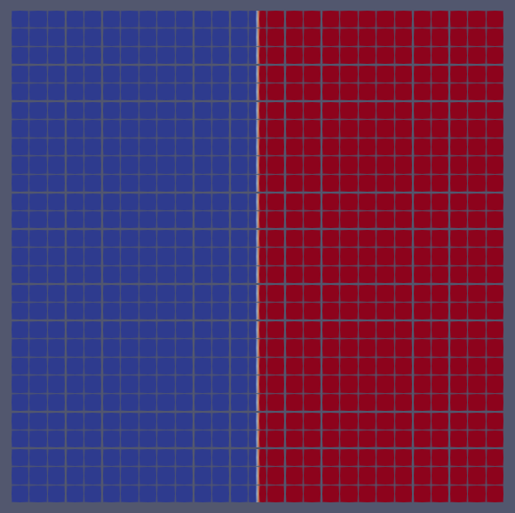
We want to simulate a so-called dam-break scenario, that is a scenario where a large mass of fluid spreads rapidly from an initial resting position, such as might happen when you jump into a pool, or when you jump into a bathtub, or when you jump into a puddle.

Exercices
1. Implement some initial conditions. Let's start simple and set all values to 0, except for the initial water height, which should be 1.0 on the left half of the domain, and 2.0 on the right half of the domain.
2. Add boundary conditions, eigenvalue and flux.
3. Run the code and visualise the outcome.

Dam break

Observations: Difference of Finite Volumes to ADER-DG

We realise that Finite Volumes and ADER-DG (as well as literally any other scheme in ExaHyPE) are really close to each other. However, the names of the parameters (as well as some parameter counts) are slightly different. This makes sense, as the parameters have slightly different semantics. The FV for example have a volume centre. The ADER-DG solver has a cell centre, and you have to puzzle out where an integration point is located within this cell - for which ExaHyPE 2 provides helper functions.

This explains once more why many codes extract their core functionality into separate classes and routines, and then let the solvers only hold the glue code. This glue code can easily be injected via Python, and the core functionality can be used by various numerical schemes. Indeed, we can have different schemes (aka solvers) in one project and couple them. They all use the same functionality albeit slightly differently.

Solutions

If you don't want to implement the routines yourself, here are the solutions (you will have to tinker around with the named variable access) and the signatures:

initialCondition( double * restrict Q, //Q[4+0] const tarch::la::Vector<Dimensions,double>& x, const tarch::la::Vector<Dimensions,double>& h, bool gridIsConstructed ) { Q[s.hu + 0] = 0.0; // v_x Q[s.hu + 1] = 0.0; // v_y Q[s.h] = x[0] < 0.0 ? 1.0 : 2.0; // h Q[s.b] = 0.0; }

boundaryConditions( const double * restrict Qinside, // Qinside[4+0] double * restrict Qoutside, // Qoutside[4+0] const tarch::la::Vector<Dimensions,double>& faceCentre, const tarch::la::Vector<Dimensions,double>& volumeH, double t, int normal ){ Qoutside[s.h] = 1.0; // h Qoutside[s.hu + 0] = 0.0; // v_x Qoutside[s.hu + 1] = 0.0; // v_y Qoutside[s.b] = 0.0; // b }

maxEigenvalue( const double* restrict Q, // Q[4+0] const tarch::la::Vector<Dimensions,double>& volumeCentre, const tarch::la::Vector<Dimensions,double>& volumeSize, double t, double dt, int normal ){ constexpr double grav = 9.81; const double u = Q[s.hu + normal] / Q[s.h]; const double c = std::sqrt(grav * Q[s.h]); return std::max(std::abs(u + c), std::abs(u - c)); }

flux( const double* restrict Q, // Q[4+0] const tarch::la::Vector<Dimensions,double>& volumeX, const tarch::la::Vector<Dimensions,double>& volumeH, double t, double dt, int normal, double* restrict F // F[4] ) { double ih = 1.0 / Q[s.h]; constexpr double grav = 9.81; F[s.h] = Q[s.hu + normal ]; F[s.hu + 0] = Q[s.hu + normal] * Q[s.hu + 0] * ih; F[s.hu + 1] = Q[s.hu + normal] * Q[s.hu + 1] * ih; F[s.b] = 0.0; F[s.hu + normal] += 0.5 * grav * Q[s.h] * Q[s.h]; }

Second exercise: Extending SWE

It is time to re-introduce the bathymetry for the second exercise:

\( @f{eqnarray*}{ \frac{\partial}{\partial t}\left( \begin{array}{lr} h \\ h u_1 \\ h u_2 \\ b \end{array} \right) + \nabla \underbrace{\begin{pmatrix} h u_1 & h u_2 \\ h u_1^2 & h u_1 u_2 \\ h u_2 u_1 & h u_2^2 \\ 0 & 0 \end{pmatrix}}_{ flux } + \underbrace{\begin{pmatrix} 0 & 0\\ h g*\partial_x(b+h) & 0\\ 0 & h g*\partial_y(b+h) \\ 0 & 0 \end{pmatrix}}_{ ncp } = \vec{0} @f} \)

Switch on the non-conservative product in your solver and implement these terms with ADER-DG. Also, you might want to change the initial conditions.

Solutions:

Again, if you don't want to implement the terms yourself, copy from here: initialCondition( double * restrict Q, //Q[4+0] const tarch::la::Vector<Dimensions,double>& x, const tarch::la::Vector<Dimensions,double>& h, bool gridIsConstructed ) { Q[s.hu + 0] = 0.0; // v_x Q[s.hu + 1] = 0.0; // v_y Q[s.h] = 1.0; Q[s.b] = (tarch::la::norm2(x) < 0.5 ? 0.2 : 0.0); }

flux( const double* restrict Q, // Q[4+0] const tarch::la::Vector<Dimensions,double>& volumeX, const tarch::la::Vector<Dimensions,double>& volumeH, double t, double dt, int normal, double* restrict F // F[4] ) { double ih = 1.0 / Q[s.h]; F[s.h] = Q[s.hu + normal]; F[s.hu + 0] = Q[s.hu + normal] * Q[s.hu + 0] * ih; F[s.hu + 1] = Q[s.hu + normal] * Q[s.hu + 1] * ih; F[s.b] = 0.0; }

nonconservativeProduct( const double *__restrict__ Q, //Q[4+0] const double *__restrict__ deltaQ, //deltaQ[4+0] const tarch::la::Vector<Dimensions, double> &volumeX, const tarch::la::Vector<Dimensions, double> &volumeH, double t, double dt, int normal, double *__restrict__ BTimesDeltaQ //BTimesDeltaQ[4] ){ constexpr double grav = 9.81; BTimesDeltaQ[s.h] = 0.0; switch (normal) { case 0: BTimesDeltaQ[s.hu + 0] = grav * Q[s.h] * (deltaQ[s.h] + deltaQ[s.b]); BTimesDeltaQ[s.hu + 1] = 0.0; break; case 1: BTimesDeltaQ[s.hu + 0] = 0.0; BTimesDeltaQ[s.hu + 1] = grav * Q[s.h] * (deltaQ[s.h] + deltaQ[s.b]); break; } BTimesDeltaQ[s.b] = 0.0; }

The above setup should yield outcomes similar to

End solution

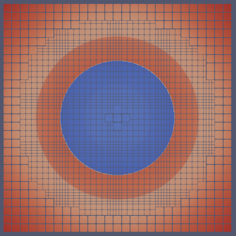
one the simulation has terminated.

Adaptivity

But there is one ingredient missing: adaptivity. All ExaHyPE solvers are, as a matter of principle, ready to support dynamic adaptivity. It is just that we haven't used it so far. We employed code snippets like the one blow in our code:

// refinementCriterion(
  const double * __restrict__ Q,               // Q[4+0]
  const tarch::la::Vector<Dimensions,double>&  x,
  const tarch::la::Vector<Dimensions,double>&  h,
  double                                       t
) {
  return ::exahype2::RefinementCommand::Keep;
}

If a solver tells Peano, the underlying AMR machinery, to keep the mesh always, the AMR environment will initially refine such that it meets your solver's maximum mesh requirements, and then that's it. To change that, let's replace this C++ code with

// refinementCriterion(
   const double * __restrict__ Q,               // Q[4+0]
   const tarch::la::Vector<Dimensions,double>&  x,
   const tarch::la::Vector<Dimensions,double>&  h,
   double                                       t
 ) {
   return (std::abs(::tarch::la::norm2(x) - 0.5) < 0.2 ?
     ::exahype2::RefinementCommand::Refine :
     ::exahype2::RefinementCommand::Keep);
 }

This is all we have to do to introduce dynamic AMR. If we return Keep for any t>0 and only evaluate this criterion for t=0, we create static AMR. Note that we don't care at all about minimal and maximum mesh sizes. Those are tied to the solver, and the engine will take care of it.