When we create hanging faces, we have to interpolate from coarse to fine.

Data storage scheme

For a setup with p volumes per coordinate axis per patch, a face always stores \( 2k \cdot p^{d-1} \) values: It stores a layer of depth k of its left neighbouring cell and a layer of the right one. These layers are copies. By separating the copies of halo layers from the actual patch data, we can easier move data around in a parallel computer. A patch only has to know some of the data from all neighbouring, face-connected patches. With our scheme, it does not need to know these neighbours at all. It is sufficient to take the faces of a cell and to use the data from there to reconstruct the actual patch plus its halo layer:

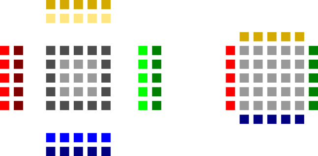
In the image above, we see a schematic illustration of the data layout: In this example, a 2d cell hosts a 5x5 grid of finite volumes and we work with an overlap of k=1. The four faces each hold 2x5 volumes. These are copies from the left and right adjacent cells. So the dark red volumes are actually copies of the volumes within the patch. In the left image, I use a darker grey to label those volumes within the patch which also have been copied by the patch onto the face.

So the four faces hold replicated data from their adjacent cells. When we want to run the Rusanov solver, e.g., we need information from the neighbouring cells. Peano does not directly use the neighbours but instead uses the replicated data from the faces to supplement the neighbour information. In this illustration, the dark data are used to re-construct the halo. Only half of the face data is used for this reconstruction. The other half is used by the respective other neighbours.

When we now look at hanging faces, we recognise that we need interpolated data from the coarser level:

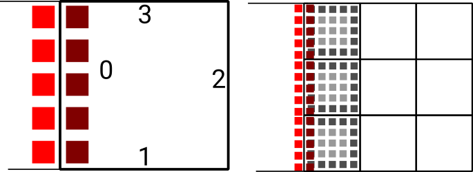
Hanging faces do not carry any information, i.e. there is no red data in the plots on the right. Only the face on the coarser level holds data. So we have to project the light red volumes down to the fine grid light red volumes, before we can update the fine grid patches (grey).

The Interpolation.h header file hosts a set of interpolation routines.

Finding the grid topology

To understand the implementation of the routines, we have to reiterate that we work cell-wisely in Peano. That is, we start from a particular cell that has a father-cell. It is one out of 3^d child cells, as we work with three-partitioning. Within this cell (which is encoded within marker as we will discuss later), we have 2d faces. If one of them is a hanging face (along an AMR transition), Peano will call an interpolation routine for it. The faces of any cell in Peano are enumerated in the same way: Face 0 is the face whose normal points along the first coordinate axis and which is left in the coordinate system. Face 1 is the face whose normal points along the second coordinate axis, and so forth. In 2d, face 0 is the left one, face 1 is the bottom one, face 2 is the right one, and face 3 finally the top face.

We can ask the marker which face we are talking about via getSelectedFaceNumber(). We can also ask the marker how this face is positioned within the grid of siblings, i.e. within a 3x3x3 grid. The routine for this is getRelativePositionWithinFatherCell(). In the example above, this routine would return (0,0), (0,1) or (0,2), respectively, Once we know the local face number and this position within 3x3x3 grid, we know the exact grid topology of a hanging face.

I originally thought I could work with interpolating only half of the halo layer. Indeed, we only have to interpolate half of the halo layer along a hanging face: the outer part. This outer data will be used to construct a halo around the adjacent fine grid patch. However, I need the interpolation of all data whenever I create a new persistent face, restricting to half of the halo does not make the code any simpler, and along the domain boundary, e.g., some routines appreciate if they have all interpolation available.

So while I could, in most cases, use the information of the normal to only write half of the halo data (for example only the bright red volumes on the fine mesh in the sketch above), I usually set all the face data on the hanging face, even though half of it is not used.

Face data enumeration

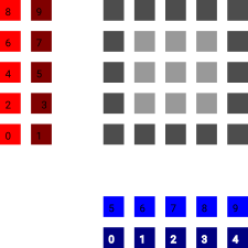
All face data are always enumerated lexicographically. That is, 0 is always the left bottom volume within the face data. Then we follow the x-axis, then the y-axis.

The image below shows the enumeration:

Interpolation as matrix-vector product

We can always interpret the interpolation as a matrix-vector product. For a system with N unknowns, it is important to recognise that we basically do the same interpolation N times. This is a batched operation, i.e. we compute

\[ u_h = P u_H \]

for N versions of \( u_h \) and \( u_H \). Peano's tarch component has a routine for batched multiplication, where you pipe in a set of \( u_H \) vectors and you get a set of \( u_h \) vectors out.

Interpolation flavours

Each interpolation type is realised via three different routes. All flavours follow the same naming convention.

Each routine starts with the prefix interpolate.
There's always one flavour that's then called interpolateCell, the other one is called interpolateHaloLayer.
I add the data storage format that underlies the operator realisation. At the moment, I only support array of struct (AoS).
The storage format identifier is followed by another underscore.
The next part of the string is the actual interpolation scheme.

We offer two types of interpolation: There's a few hard-coded interpolation schemes which are written in core C++ and realise the interpolation. There is also a generic verison of the interpolation which expects the user to pass in an interpolation matrix and then applies this matrix instead of a hard-coded operation.

If you work with the generic implementation accepting matrices, then most codes pre-compute the required matrices manually (within a Python script, e.g.) and then pass in a pointer to a constant double field holding the matrix. Please consult toolbox::blockstructured::interpolateHaloLayer_AoS_generic() for details.

Technically, there are always two types of interpolation routines per face: There is a version which is given the coarse cell face only. I use this one to interpolate from a coarse level onto a face at the boundary of a finer \( 3 \times 3 \) patch. The other variant of the interpolation is used for an interior face within a \( 3 \times 3 \) patch and is also given the coarse cell data. The latter variant is only called to create new faces. It is never used for hanging faces.

For this one, I have to create the fine grid volumetric data, and then copy the interpolated data from there onto the face data. This way, we are consistent with the idea that face data always holds copies from adjacent fine grid data.

Caching of inter-grid transfer operators (only for built-in C++ operators)

Constructing the interpolation operators can be time consuming. I therefore cache the operators.

For the handling of faces at the boundary of the \( 3 \times 3 \times 3 \) patches, I hold one large interpolation matrix per normal. So for 2d, I have four interpolation matrices, for 3d I have six. The large interpolation matrix per direction can compute all \( 3^{d-1} \) faces in one rush, so we usually only need one out of them at a time. So I have this huge map with these matrices. When we have to interpolate, we first check whether we've already assembled the matrix. If so, we use this one. If not, we first compute it and cache it in the map.

For the volumetric interpolation and the handing of the interior faces, we use another map. That is, if we want to compute the interior face, we first project onto a temporary \( 3^d \) set of volumes, and then we extract the fine face data from there. This implies that we are consistent with the actual projection of face data, where we take fine grid volume values and write them onto the face data as copies.