 |
Peano
|
|
Peano
|
ExaHyPE's discontinuous Galerkin realisation provides support for plain higher-order DG with Riemann solvers of your choice.
The C++ code is a mere collection of routines. It is rather a toolbox than a real solver. It is the Python code which serves as glue. It takes the individual events triggered by Peano's mesh traversal, augments it with ExaHyPE-specific data structure, and maps it onto DG routines. Furthermore, the generated Python code holds all the DG matrices and vectors. These are not hardwired into the C++ routines but passed in as arguments (pointers). The mapping from the traversal events onto DG computations is realised via action sets. This is the Peano terminology.
We rely on the generic DG formulation for
\( \partial _t Q(t) + div F(Q(t)) = S(Q(t)) \)
which is subject to a weak formulation. A discussion of non-conservative terms can be found further down. For the time being, we focus on a conservative formulation and examine the weak formulation which has to hold for any reasonably smooth test function \( \phi = \phi (x)\):
\( \int _{\Omega } \left( \partial _t Q(t), \phi \right) dx + \int _{\Omega } \left( div F(Q(t)), \phi \right) dx = \int _{\Omega } \left(S(Q(t)), \phi \right) dx \)
In the DG framework, any test function \( \phi \) has strict local support which reduces the weak formulation to a cell expression: We know that \( \phi \not= 0 \) inside one specific cell c, but it equals zero everywhere else. Within this one cell, our shape function is continuous. Therefore, we can apply integration by parts and the product rule for divergence and obtain
\( \int _c \left( \partial _t Q(t), \phi \right) dx - \int _c \left( F(Q(t)), \nabla \phi \right) dx + \int _{\partial c} \left( F(Q(t)), \phi \right) dS(x) = \int _c \left(S(Q(t)), \phi \right) dx \)
It doesn't really matter for the discussion here how we treat the time derivative. Our discussion focuses on how we compute \( \partial _t Q \) and it is then up to your time integrator of choice how to process this information further. From hereon, any reference to \( \partial _t Q \) means we speak about the change of the value in time for one particular quadrature point, i.e. one particular weight.
In ExaHyPE 2, we mainly use Runge-Kutta. If the weak formulation is subject to Runge-Kutta, we evaluate a series of forward shots/trials and then combine these shots finally into the new solution. All we need is a description of the time derivative, which we obtain from the weak formulation above. As our C++ toolbox is independent of the time integration scheme used, I decided to place it in a namespace dg, whereas the Python glue code might have different namespaces reflecting different timestepping schemes.
On this page, I do not discuss Discontinuous Galerkin in detail, but I try to point out, how the individual steps are integrated into the mesh traversal, and how I split them up into individual routines.
We solve
\( \int _c \left( \partial _t Q, \phi \right) dx = \int _c \left( Q, \phi \right) dx + dt \cdot \left( \int _c \left( F(Q), \nabla \phi \right) dx - \int _{\partial c} \left( F(Q), \phi \right) dS(x) + \int _c \left(S(Q), \phi \right) dx \right) \)
Which is just one step of the forward euler method with the time derivative from above. ExaHyPE works with cubic or square cells and a Cartesian layout of the degrees of freedom therein. We thus have \( (p+1)^d \) degrees of freedom in our square/cube cells. Each carries n unknowns, but they are all treated the same, i.e. independent of each other. So it is sufficient to look at one unknown. We may assume that the Q is scalar. The F and S term can potentially couple n unknowns per dof from the previous time step with each other. But this is irrelevant to the formulation of the problem.
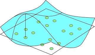
Each of the \( (p+1)^d \) unknowns carries one shape function. The picture above illustrates this: There's a polynomial which is tied to one particular dof and this dof holds a weight, i.e. a scaling of this one shape function. The test functions \( \phi \) are polynomials, too. All of these polynomials live only within one cell. The solution is then actually a combination of all of the polynomials scaled by the dof weights. In the sketch, the solution is a linear combination of 16 polyomials within this very cell. Then it might jump on the cell face, and in the next adjacent cell there are another 16 dofs which determine the solution's shape.
As the integrals of the weak formulation span one cell only, we get something like
\( M \Big( \partial _t Q \Big) = \Big( ... \Big) Q^* \)
per cell. There is a square mass matrix which results from the integral above which tells us that a linear combination of the derivatives within a cell equals an expression over all previous values of the time step. This is the reason I add the star. It is just there to point out that we use a lot more values than only those within one cell.
The M is the MassMatrix. Let all the dofs within a cell be enumerated lexicographically. Each value scales the underlying shape function. The first line of the mass matrix then tells us what the linear combination of all of these shape functions scaled by the weights and tested against the first gives under the integral. The second line of the \( M Q^{(new)} \) tells us what the test of the linear combination against the second test function gives us.
We can compute the mass matrix a priori. This is done by the Python script exahype2.solvers.LagrangeBasisWithDiagonalMassMatrix for example. The computed matrix is then written into the abstract solver base class of the user and can be handed over to any computational routine. We note that we will (more often) need the inverse.
\( \partial _t Q(T) = M^{-1} \Big( \dots \Big) Q^* =: Q + dt \cdot M^{-1} \hat Q\)
This is the last step of our algorithm: We assume that we have a quantity \( \hat Q \) in each and every sample point whose entries will be discussed later. We multiply these quantities with the inverse of the mass matrix and add it, subject to a scaling with dt, to the old solution. This operation is called exahype2::dg::multiplyWithInvertedMassMatrixAndAddToSolution_GaussLegendre() or variants thereof. So far, the algorithm thus consists of two steps:
You will find exahype2::dg::multiplyWithInvertedMassMatrixAndAddToSolution_GaussLegendre() and its cousins in the file exahype2/dg/CellIntegral.h as they correspond, as name and derivation suggest, to an integral formulation over integrals.
You can pick different shape functions. For different shape functions, you get different mass matrices. \( M \) in general is a dense matrix. Its entries stem from
\( M_{ij} = \int _c \Big( \phi _i, \phi _j \Big) dx \)
For some (approximations of) mass matrices or particular choices of the shape fuctions, we provide specialised versions of DG's mathematical steps. All mass matrices have in common that the underlying shape functions have local support. They never extend beyond a cell. Therefore, mass matrices are always square and have exactly \( (p+1)^d \) rows/columns.
Important special cases of mass matrices arise if some of the following properties hold:
As we use Discontinuous Galerkin where the individual shape functions are confined to a cell, M couples really only dofs of one cell with each other. There is no reason to use a lumped matrix as the (global) inverse then also has block structure, i.e. couples only dofs from within one cell. But some codes might nevertheless prefer lumped (diagonalised) matrices for performance reasons.
Purists might argue that most setups don't need the inverse of the mass matrix, as the mass matrix inverse coincides with the mass matrix inside the \( \hat Q \) term. However, there are cases where this is not the case, and if you know that your mass matrix is a diagonal, then we offer specialised versions for this anyway, and you can afford the few additional multiplications that result from the fact that our \( \hat Q \) is the result of the test and we do not mangle in the inverse of the mass matrix a priori.
From the definition above, we note that the ith entry of \( \hat Q \) denotes what happens if we have a global solution Q and test it against the test function \( \phi _i \) carried by this ith dof from a cell. The computation of this intermediate value \( \hat Q \) consists of two types of contributions: Contributions from the face integrals and contributions from the volumetric terms. I discuss the terms individually and split any term discussion again up into two parts if a term arises under the surface and the volume integral.
This is different to the implementation where you find a routine cellIntegral_patchwise_GaussLegendre_functors() or any of its cousins which does all the volumetric stuff in one rush, while the handling of the face contributions is done differently.
In ExaHyPE's DG code, we distinguish two types of source terms: Volumetric source terms and point sources. Usually, I mean volumetric source terms when I speak of a source.
Once we assume that S(Q) is something that exists in each and every point within the domain, we have to make a decision how to represent it as a function. It is convenient to assume that S can be represented in the same way as the solution Q, i.e. as linear combination of the same type of shape functions.
In this case, we obtain a matrix-vector product
\( M\dot S(Q) \)
when we integrate over \( (S,\phi ) \). If we insert this formalism into the equations above, we recognise that we would never need the outcome of the matrix-vector product. Instead, we are interested in
\( dt\cdot M^{-1}M\dot S(Q) = dt\cdot S(Q) \)
in the end. However, I made the design decision that I want to have these steps as proper separate steps. The reason is that we have to treat some other terms differently:
Point sources are modelled as Dirac terms within S:
\( \int _c \Big( \delta _p, \phi \Big) dx = \phi (p) \)
So we basically get, for a test with a test function \( \phi \), the value of this test function at the point source (times a calibration if the point source should not be one). Our implementation runs over all point sources within a cell. As we know that the test functions span only the current cell and disappear everywhere else, we don't have to check all point sources out there. Per point source, we test over all the \( (p+1)^d \) test functions associated with the dofs of this cell, and add the corresponding values to \( \hat Q \).
The source term solely enters the volumetric calculations. It does not show up in any face integral. With source terms, our algorithm implementation consists of the following steps:
A final consideration is that for higher dimensions the shape functions' tensor-product structure can be exploited to obtain higher order mass matrices \( M_{2d} = M \otimes M \) and \( M_{3d} = M_{2d} \otimes M \).
As any shape function has local support within one cell, we can evaluate per cell by employing integration by parts:
\( \int _c div F(Q(t))\ \phi dx = - \int _c \Big( F(Q(t), \nabla \phi \Big) dx + \int _{\partial c} F(Q(t)) \ \phi \ n dS(x) \)
The volumetric integral looks complicated, but it can be broken down into simpler steps. First, we consider a one-dimensional setup. Let us assume that we can represent \( F(Q) \) once again with our shape functions. That's not point-wisely true usually, but we can work with this assumption. If this is the case, then the \( F(Q) \) can be written down as an evaluation of the Fs in the quadrature point, and then we can take the outcome and interpret it as weight of the shape functions. So we get expressions like
\( \int \Big( F(Q(x_i)) \phi _i, \nabla \phi _j \Big) dx \)
which are then linearly combined to give us the integral. We now observe that we know the test functions, i.e. we can also precompute the derivative. Furthermore, we can move the weight out of the integral. This gives us
\( F(Q(x_i)) \int \Big( \phi _i, \nabla \phi _j \Big) dx = D F(Q) \)
where the matrix D is the StiffnessOperator which is the product of quadrature weights and the integral over the test functions and its derivative. Q is the vector of the unknowns.
If we have a a two-dimensional problem, we note that we benefit from the tensor product structure once again. As
\( \phi (x,y,z) = \phi (x) \cdot \phi (y) \cdot \phi (z) \)
decomposes the function into a product of independent ones, we can also decompose the integral:
\( \int \Big( F_x(Q(x_i,y_i)) \phi _i, \nabla _x \phi _j \Big) d(x,y) = F_x(Q(x_i,y_i)) \int \Big( \phi _i(x)\phi _i(y), \nabla _x \phi _j(x)\phi _j(y) \Big) d(x,y) = F_x(Q(x_i,y_i)) \int \Big( \phi _i(x), \nabla _x \phi _j(x) \Big) dx \int \Big( \phi _i(y), \phi _j(y) \Big) dy \)
which are then linearly combined to give us the integral. In the generic case, we will need to make D a \( (p+1)^d \times (p+1)^d \) matrix. If we have Gauss-Legendre polynomials however, we can once again exploit the fact that the polynomials are orthogonal. It is hence sufficient to have a one-dimensional \( D_{1d} \) diffusion operator and the one-dimensional mass entries to construct all diffusion operators.
More specifically, this higher dimension form can be split into the product of a mass matrix and a stiffness matrix. WHen considering the flux along the x-axis, the mass matrix is applied along the y-axis and z-axis, so we can calculate the relevant matrix as \( M_x = M \otimes M \otimes I \). The stiffness matrix is only applied along the x-axis, so it can be calculated as \( K_x = I \otimes I \otimes K \). The final contribution from the flux along the x-axis is then \( h(1) \cdot h(2) \cdot MKF(Q) \).
The scaling of the volumetric contribution is in \( h^{d-1} \). We have a \( h^d \) from the integral, and we have a \( h^{-1} \) from \( \nabla \phi \). The source term solely enters the volumetric calculations. It does not show up in any face integral. With source terms, our algorithm implementation consists of the following steps:
ExaHyPE uses a nodal approach, in which the value stored for each dof is the true value at that quadrature point. The shape functions operate as interpolating polynomials between the quadrature points. This differs from a modal approach, where a linear combination of all shape functions must be taken to obtain the value at any point. This means that the source and flux values can be easily obtained like in other schemes.
The spacing of the nodes is not necessarily equidistant. We obtain better accuracy using Legendre nodes, which are the roots of the Legendre polynomial of order \( p \). The Lagrange polynomials which we use as shape functions are not necessarily orthogonal, so we may not have a diagonal mass matrix. However, we do if we use Legendre nodes. We could also use Gauss-Lobatto nodes, which would not lead to a diagonal mass matrix, but would simplify the projection onto faces.
To apply any Riemann solver of our choice, we first have to project the current solution \( Q(t) \) from within the cell onto the faces. This projection is realised by a dedicated Python action set which is fed the polynomial basis functions.
We can exploit the fact that we employ Lagrangian basis functions and that we also work with Cartesian tensor product structures. Due to these choices, we know that any projection of the current solution representation within the cell can be mapped onto a Lagrangian polynomial of exactly the same order on the face. Furthermore, everything is beautifully lined up: In 2d, all the integration point within a cell along a horizontal line span up a polynomial, and we can thus multiply them with this polynomial and thus reconstruct the polynomials value on the left and right faces' sample point (which also is exactly on this line). We don't even have to use Gauss-Lobatto points. It works with Gauss-Legendre just as well (with Lobatto, we could avoid the construction of the polynomial and just read out the solution value right at the face; we do not yet exploit this fact).
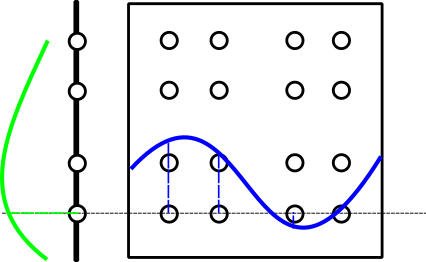
In the 2d example above, the four bottom sample points and their weight define the blue polynomial along the horizontal line. The other 12 integration points in the cell have no influence on the solution value along this line because the Lagrange polynomials are 0 there. Consequently, we can compute the left and right solution solely by these four weights.
On the left face, we have a polynomial with the same order (3rd order here), but it is - obviously - a 1d polynomial and not one resulting from a tensor product. Once we know the the volumetric polynomials value on the left face, we can directly set this value as weight on the face's quadrature point (green weight).
Each face has a left and a right side, and the solutions left and right will not be the same as we work in a Discontinuous Galerkin setup. We hence do not store four weights in the example above, but we do hold eight weights, i.e. both the weights from the left and the right side. These weights are stored lexicographically in line with the Finite Volume solver. See the documentation of the face enumerator exahype2::enumerator::FaceAoSLexicographicEnumerator. In the vanilla version of ExaHyPE, we do only store the solution left and right. For more sophisticated Riemann solver, you can also store derivatives, e.g., from both sides.
The projection onto the faces is an operation within the polynomial function space. As there's no integral or something similar involved, it is a plain multiplication of the sample points' weights within the cell with the corresponding weights of the polynomial.
\( \int _{\partial c} F(Q(t)) \ \phi \ n dS(x) \)
requires work (and care), as Q (and hence F) are not defined on the cell faces. We therefore have to approximate the physical flux F by a numerical flux, there are several definitions for numerical fluxes, but one generic way to tackle this is to exploit standard Rusanov, e.g. In this case, we employ some averaging of the faces subject to additional damping.
\( \int _{\partial c} F(Q(t)) \ \phi \ n dS(x) \mapsto \int _{\partial c} \Big( \frac{1}{2}(F(Q^-(t))+F(Q^+(t))) - \frac{1}{2} \lambda _{max}(Q^-(t),Q^+(t)) (Q^+(t)-Q^-(t)) \Big) \ \phi \ n dS(x) \)
This is what we do when we touch a face. We simply take the projected Q values from left and right and compute what F looks like. In theory the solutions to the left and right of the face could be different. Therefore we hold both outputs.
Let the outcome of a Riemann solve (the solution) be the thing under the face integral without the \( \phi \) test function. For the Rusanov example above, we would call the result of
\( \frac{1}{2}(F(Q^-(t))+F(Q^+(t))) - \frac{1}{2} \lambda _{max}(Q^-(t),Q^+(t)) (Q^+(t)-Q^-(t)) \)
the solution to the Riemann problem. This is essentially a numerical approximation of the physical flux between neighbouring volumes (and therefore cells.)
Once we know the point-wise Riemann solution, we know that this point-wise solution spans functions in the shape space restricted to the faces. That is, the individual points of the Riemann solution serve as weights to shape functions which live on the face only. We can analytically integrate over these (we know the shapes and have a linear combination) and then project the data back. Once again, the integral is the mass matrix, though this time a mass matrix on the submanifold. It has a scaling of \( h^{d-1} \).
Every single test on the face is the result of a projection of a volumetric test function onto the face. This explains how the outcome affects the \( \hat Q \): We simply take the outcome and distribute it according to the original projection matrix. Mathematically this equals a multiplication with the transpose. There's no scaling involved in this step anymore.
The whole algorithm implementation hence reads as follows:
You find some discussions of the treatment of the non-conservative product in papers by Michael Dumbser et al, e.g. I found the discussion around \( P_NP_M \) patch-conservative products in his paper "Space-time adaptive ADER discontinuous Galerkin schemes for nonlinear hyperelasticity with material failure" particularly helpful (arXiv:2003.02760). Have a look notably into (21). Other useful sources of information can be found in this presentation, e.g.
Personally, I always use the following hand-wavy explanation:
We usually keep the \( B_x(Q)\nabla _xQ \) term as it is and assume that we can represent the outcome again in the same polynomial space that we used for the shape functions. This is quite a crude approximation, as the ncp terms can be really non-linear and nasty, so it is unlikely that the analytical solution can be represented by the same linear combination of shape functions as the input. But we don't really know that much about the ncp term anyway, so any other choice of shape functions to represent the outcome would be equally flawed.
If the \( B_x(Q)\nabla _xQ \) term projects into our ansatz space, then the whole ncp contributions enter our equations as one giant mass matrix times B(Q). However, that's only a part of the story.
Whenever we study
\( \int _\Omega \Big( B_x(Q)\nabla _xQ, \phi \Big) dx \)
we know that we can split up the integral into a sum over integrals over the cells but that the faces require special care, as the solution jumps there. In the context of the ncp, we follow the argument by Hulsen et al: The idea is that we split up the integral domain into two areas: The face plus and \( \epsilon \) environment and the remainder of the cells. So we get a sum over the faces (plus the tiny area around them) and the remaining cells. We have already discussed the latter. Here, we obtain a mass matrix.
In this \( \epsilon \)-environment around the face, now approximate \( Q \) with a continuous function. So we interpolate between \( Q^- \) and \( Q^+ \). As we make \( \epsilon \) smaller and smaller, the interpolation approximates the jump between \( Q^- \) and \( Q^+ \) better and better. The literature makes quite a lot of fuzz about pathes here and path-conservative integrals, but really most of the time it is sufficient to think of it as an interpolation which smoothes out the jump.
We end up with an integral
\( \int _{\partial c^{\epsilon}} \Big( B_x(Q)\nabla _xQ, \phi \Big) dx \)
where the \( Q \) once more is not properly defined. In line with the Rusanov approximation, we assume that Q is roughly the average when we evaluate B, i.e. we evaluate the term
\( B_x(Q) \mapsto B_x \Big( \frac{1}{2}Q^- + \frac{1}{2}Q^+ \Big) \)
In the implementation, we note that we now use the term B in two different scenarios: As an application to the gradient and as an application to the average. Obviously, it makes no sense to ask users to provide B twice (they are exactly the same operator), so we call the argument always gradient in the implementation but in the boundary context, we hand the average into the function.
The gradient at the cell interface is not known, but we can approximate it with a standard finite differences formulation where h is the volume size along the coordinate axis:
\( \nabla _xQ \mapsto \frac{1}{h} \Big( Q^+ - Q^- \Big) \)
So far, we still have a volumetric formulation, where the \( \phi \) term either picks the right or the left half of the term. This yields another factor of 0.5. We finally integrate along the normal to obtain a face integral in line with the flux term, i.e. we get a real integral over the face but the 1/h term is eliminated by the integration. We end up with
\( \int _{\partial c^{\epsilon}} \Big( B_x(Q)\nabla _xQ, \phi \Big) dx \mapsto \pm \int _{\partial c} B_x \Big( \frac{1}{2}Q^- + \frac{1}{2}Q^+ \Big) \frac{1}{2} \Big( Q^+ - Q^- \Big) \ n dS(x) \)
Usually, the
\( B_x \Big( \frac{1}{2}Q^- + \frac{1}{2}Q^+ \Big) \frac{1}{2} \Big( Q^+ - Q^- \Big) \)
is expressed in terms of the shape functions projected onto the faces. As we follow a tensor product ansatz, we obtain a d-1-dimensional mass matrix that has to be applied to the face values.
Even though we try to separate the spatial from the temporal discretisation, it is the Runge-Kutta DG scheme which is currently the most mature version within ExaHyPE 2. The main data format discussion, i.e. what do we store where and when, can thus be found in the python subdirectory
exahype2.rkdg
and the class
exahype2.rkdg.RungeKuttaDG
which serves as base class for different implementation variants. The base class mainly creates the data structures (a polynomial per cell, the polynomial's projections onto the face, all meta data, and the intermediate solutions for the Runge-Kutta scheme) and defines all potential operations on these meta data, i.e. all the glue code linked to the present C++ routines.
It is however the job of the Python subclasses to switch the individual actions on or off per grid sweep. While the Python docu provides more details on the actual behaviour of the actions, the present file discusses some of the elementary steps needed by any time stepping scheme, and which routines in C++ realise these steps. That is, we discuss how things are implemented and what they do, but we leave it to Python to orchestrate when these steps are actually done.
 1.9.8