This documentation is autogenerated from ./tutorials/mghype/examples/11_petsc-cg.ipynb. Once you clone the Peano repository, please work against this notebook or study Peano's generic description how to generate web docu from Jupyter notebooks.

This tutorial runs through the basic steps of any multigrid application. For this, we assume that you have followed the installation instructions already. We furthermore assume that the following extensions have been added: –enable-blockstructured –enable-particles –enable-loadbalancing –enable-finiteelements –enable-mghype –enable-exaparty –enable-exahype If you have a parallel code, you furthermore need –enable-loadbalancing This is for domain decomposition as we discuss later. Typically, we kick off with a new director for our project. Within this directory, we start with a plain Python script. In this guide, we work with a Jupyter notebook rather than a script. MGHyPE codes need to know where to find the MGHyPE and Peano Python sources. For this, we can either add the Python sources to our environment, or export the path variable prior to invoking our script/kicking off our Jupyter notebook, or we set the path hard-coded in our script. To be honest, this last approach is likely the least elegant one, as it hard-codes the pathes, but it works:

import sys, os
 
sys.path.insert(0, os.path.abspath("../../python/"))
sys.path.insert(0, os.path.abspath("../../src/"))

Our code atm is not super-clean. On the long run, we want to hold all codes, i.e. C++ and Python, within the src directory. For historical reasons, we still have the C++ code mainly in src, and the majority of the Peano code base in python. Only the multigrid Python ingredients are already moved over into src.

Once we have ensured that all pathes are correct, every project built with MGHyPE starts with the same imports:

import peano4.api, mghype

peano4.api

Definition __init__.py:1

Peano 4 (C) www.peano-framework.org
VTK is not available, not loading peano4.api.visualisation.
ParaView is not available, not loading peano4.api.visualisation.
Peano 4 - Multigrid extension

At the moment, we get a lot of warning from this box. They stem from the fact that a lot of our documentation uses LaTeX formulae. Python doesn't care (they are embedded into strings), but Jupyter is a little bit picky.

An MGHyPE project and its lowering into a Peano project

Every MGHyPE project defines a sequence of lowering steps. That is, we start with an MGHyPE project object. This represents the domain level, where we do the math. After that we lower this project into a Peano project. This is a technical representation (still in Python) of the arising algorithm, i.e. something that represents the actual code base realising our domain knowledge. Then we ask Peano to lower this project into native C++ code plus a Makefile.

Lowering process

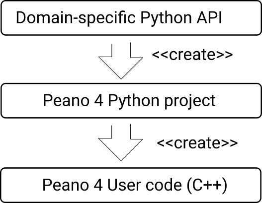
The term lowering stems from the compiler community where they use it to argue about different domain-specific languages and their abstraction levels.

project = mghype.matrixfree.api.Project( project_name = "MyProject", 
                              namespace = [ "tutorials", "mghype" ]
                            )

project.subdirectories =  ['']

This creates the domain-specific project. What follows is the lowering. This lowering happens at the end of the setup script typically. We demonstrate it once here to explain the process, even though this will give us a totally empty meaningless project, as we haven't yet added any domain-specific logic:

project.set_Peano4_installation( "../..", peano4.api.output.CompileMode.Asserts )
 
peano4_project = project.generate_Peano4_project()
peano4_project.generate()

AttributeError Traceback (most recent call last)

Cell In[5], line 3 1 project.set_Peano4_installation( "../..", peano4.output.CompileMode.Asserts ) -—> 3 peano4_project = project.generate_Peano4_project() 4 peano4_project.generate()

File ~/git/Peano/src/mghype/matrixfree/api/Project.py:166, in Project.generate_Peano4_project(self, verbose)
    154   def generate_Peano4_project(self, verbose=False):
    155     """!
    156 
    157 Build project
   (...)
    161      
    162     """
    163     self._project.main = MatrixFreeMain(self._project,
    164                                 self._domain_offset,
    165                                 self._domain_size,
--> 166                                 self._plot_each_timestep,
    167                                 self._max_iterations
    168                                 )
    170     self._project.solversteps.add_step(self.algorithm_step_create_grid)
    171     self._project.solversteps.add_step(self.algorithm_step_init_solution)


AttributeError: 'Project' object has no attribute '_plot_each_timestep'

We first get some output that stems from the set_Peano4_installation() call. This one parses all the flags you handed into CMake or the configure script, respectively, and picks them up. It also looks which static libraries have been built and so forth. So from hereon, the project "knows" what your installation looks like. It will also run some primitive sanity checks to see if all the required extensions are activtated.

Once completed, we lower the domain-specific object into a Peano 4 object. We can still add further content on this abstraction level (e.g. external libraries can be added here), but eventually we call generate(). This makes the code dump a lot of glue file which is at this point largely empty, as we haven't added any functionality yet. Later on, the code will automatically befill them with something meaningful. We end up with a complete C++ code base with all of our functionality plus a plain old Makefile to build our actual code:

!ls

generic-mixed-DG.dox   hitchhikers-guide.ipynb  matrixfree  tutorials.dox
hitchhikers-guide.dox  illustrations        petsc

shows us that we now have a Makefile, which we can either use on the command line, or we trigger the make from through a Python subprocess call. The generated code that is now scattered over all the generated subdirectories follows the generic Architecture of any code built on top of Peano:

System architecture

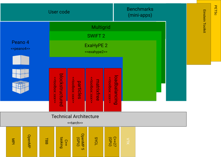
A domain-specific code sits on top of some extensions plus the Peano core, and all of the components use a common technical architecture. Third-party libraries are either hidden by the tarch, or they are plugged into the domain-specific code. We don't use any so far.

Add the functionality

Every single multigrid project adds solvers before it lowers the project into a Peano 4 project, and also sets some simulation parameters:

cube_size = 1.0
dimensions = 3
project.set_global_simulation_parameters(
  dimensions            = dimensions,
  offset                = [ 0.0       for _ in range(dimensions) ],
  domain_size           = [ cube_size for _ in range(dimensions) ],
  plot_each_timestep    = True,
)

but these topics are now covered in the individual subtutorials.

Visualisation

Peano writes its own bespoke data file format. There are some scripts delivered to convert them into VTK which you can load into Paraview or VisIt, e.g. A lot of applications also provide their own scripts to analyse the output. In theory, you can embed all of this postprocessing into Jupyter notebooks, too. With Paraview, this can be a little bit fiddly. With other postprocessing, the normal workflow is that you build the code (see remark on Make above), then you run the code on the terminal through the Python notebook (cmp the use of the ls command above) and you pipe the outcome into a text file. You can then invoke the data postprocessing scripts of your choice directly within the notebook on the dumped file and plot the outcome in-situ.